Chapter 6 Pre-test Questionnaire- Factor analysis
In this stage, the main idea is to analyze the presence of latent variables or how the questions are grouped together in clusters. With regard to latent variables, the previously defined concepts could be useful. Thus, with factor analysis, it is expected that latent variables represented by factors could identify these concepts; and questions linked with the same concept were grouped together. One of the main objectives of the factor analysis is to associate each item with only one factor. Besides, it is expected that this factor, aggregating several items, has a relevant meaning that encompass the significance of the items involved; which in the end is the latent variable.
After considering the analysis of both, the pre-genomic test and post-genomic test questionnaire, and having identified potential items to be excluded, the factor analysis is performed to finally determine which items to hold and which to exclude. Therefore, first expectations items are analyzed in both settings the pre and post-genomic testing. Then attitudes items are evaluated, again, in both the pre and post genomic instance.
6.1 Expectations and concerns domain
6.1.1 Including all the items.
The first analysis will be done for expectations items plus concerns in order to explore the relationship between all the items. Then, the analysis will be performed excluding different candidates items to find the best combination of the whole expectations and concerns domain. In this first analysis, item 4 is considered inverted.
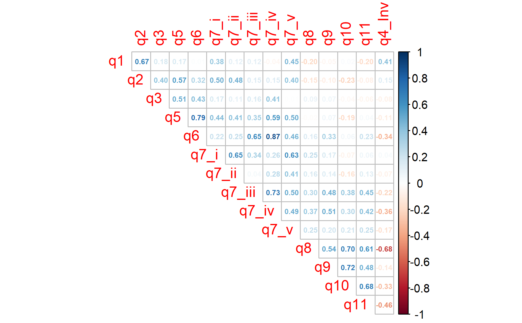
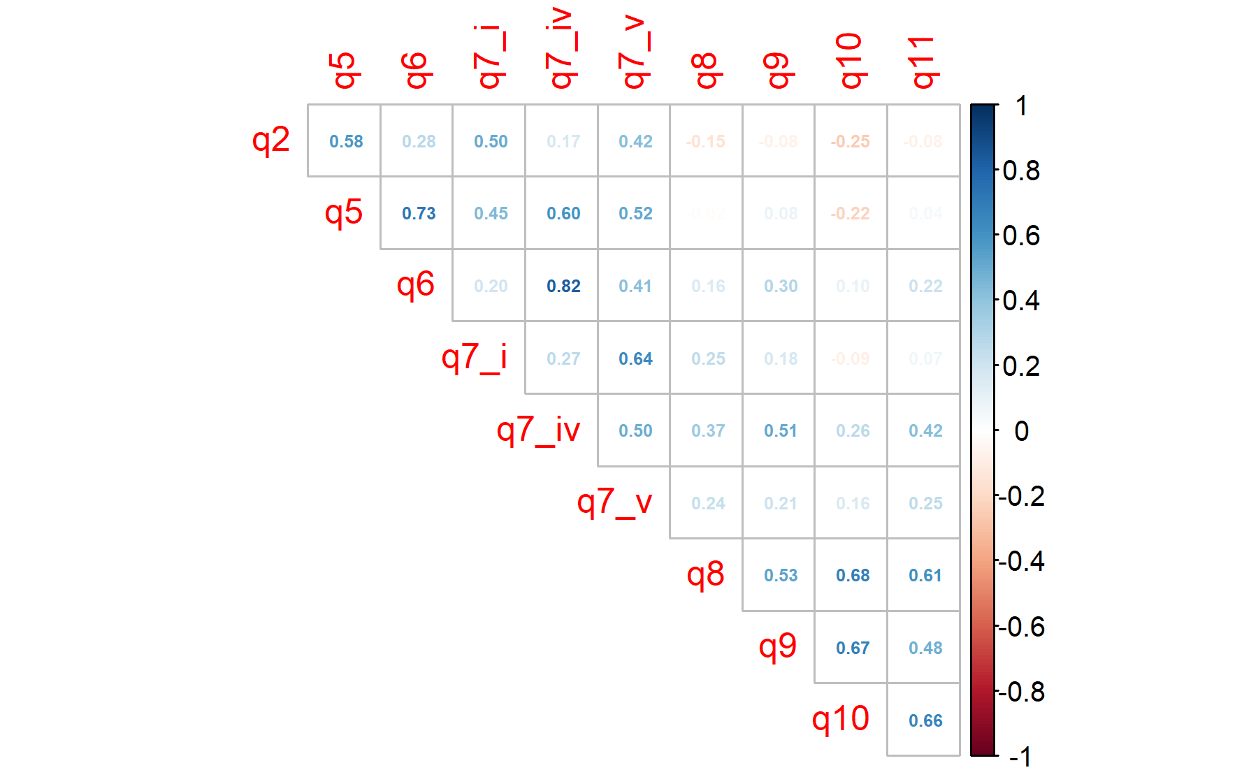
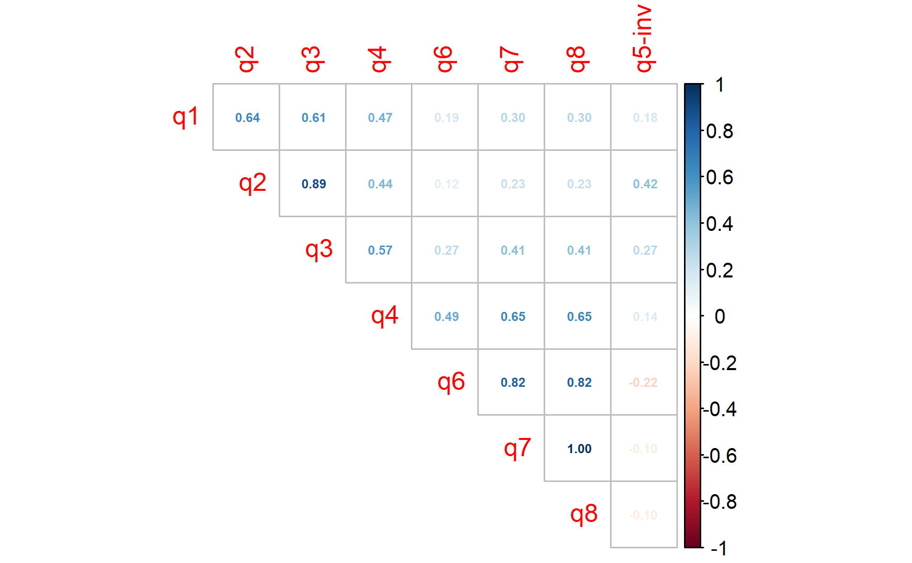
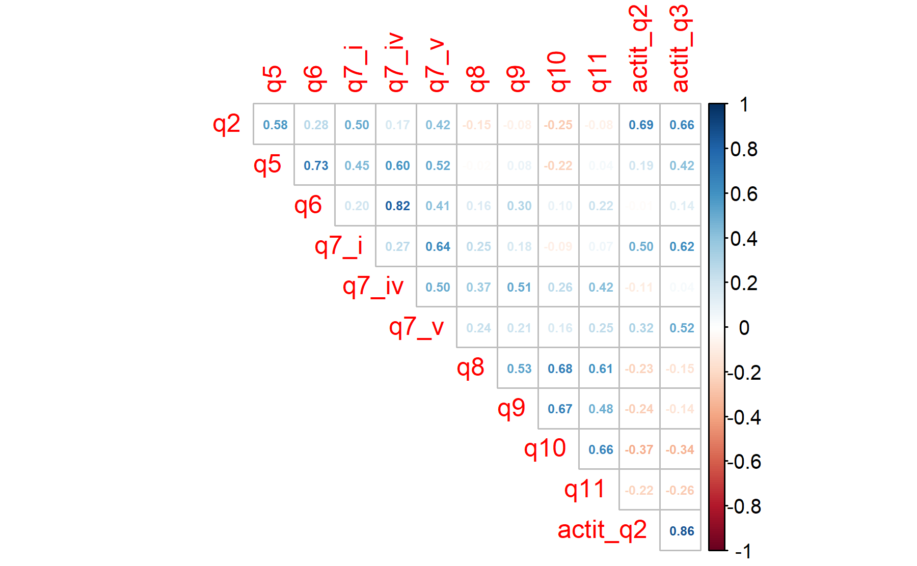
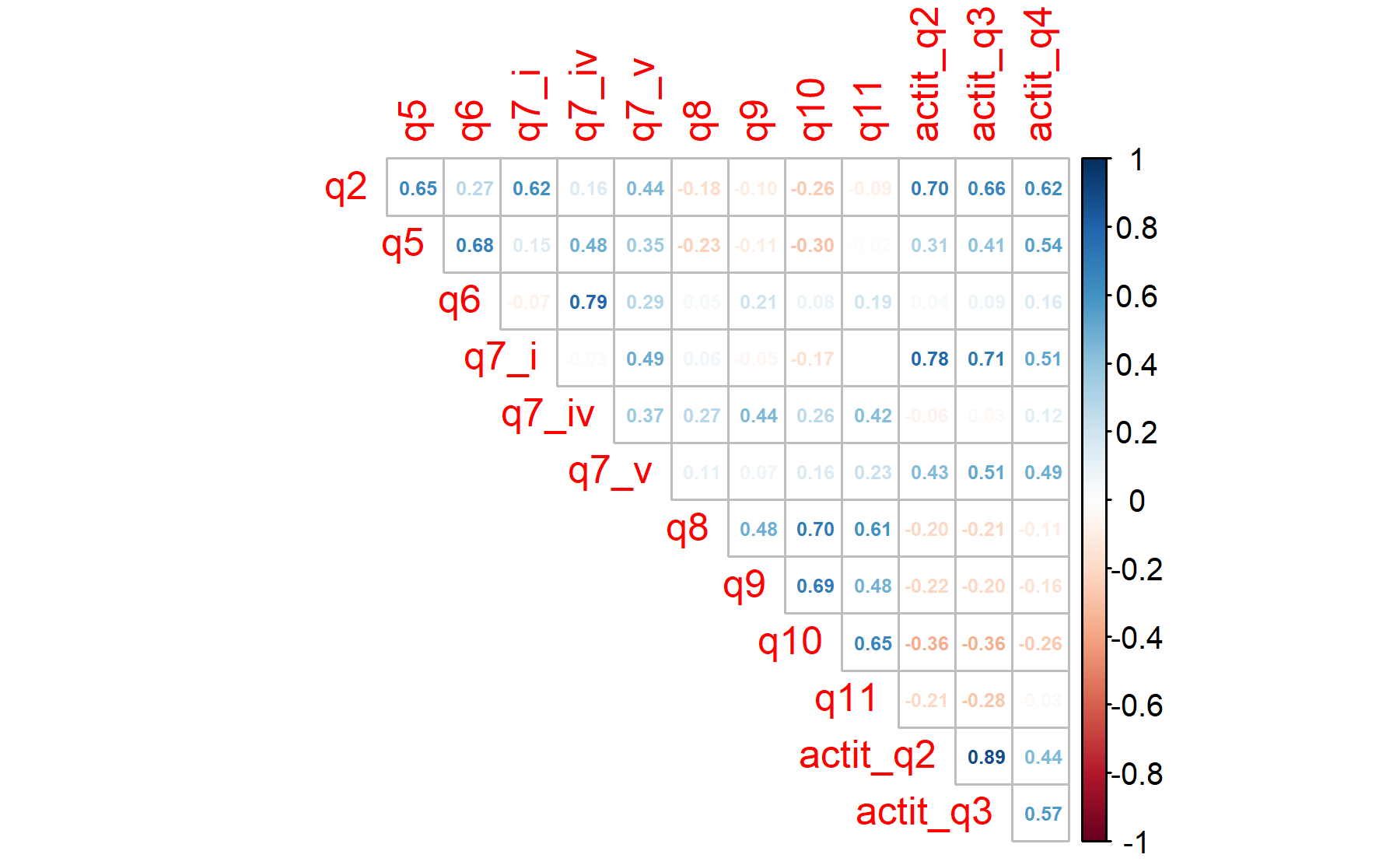
Figure 6.1: The list of the items are: 1.Tengo suficiente conocimiento de beneficios y riesgos para tomar decisión informada, 2.He recibido suficiente información para comprender beneficios y riesgos del análisis genómico, 3.Estoy interesado/a en aprender más, 4.Necesito visita formal con especialista consejo genético antes del test, 5.El resultado ayudará al control de mi cáncer, 6.El resultado ayudará a aumentar mi expectativa vida, 7i.Mi Dr me explicará resultados y la implicación para mi salud, 7ii.Recibiré informe escrito con el resultado, 7iii.Mi Dr cambiará mi tto de acuerdo a los resultados, 7iv.Tendré opciones de tratamiento adicionales, 7v.Podré recibir tratamientos experimentales, 8.Me preocupa que los resultados puedan no guiar mi tratamiento, 9.Me preocupa que los resultados pueden ser difíciles de comprender, 10.Me preocupa que los resultados pueden dar información del riesgo de enf que preferiría no saber, 11.Los resultados pueden preocuparme o generar ansiedad
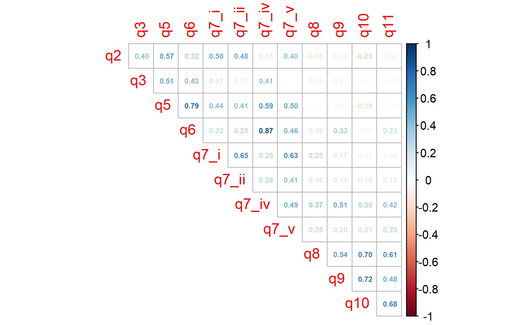
There is some consistency between correlations, at least with most of them. For instance, between Q1 and Q2; Q5 and Q6; Q6 with Q7iii and Q7.iv; and the relationship between Q8-q11. Besides, the Q4 inverted has a moderate correlation with Q1.
As first approach the Barlett’s sphericity test is performed.
Bartlett’s sphericity test provides information about whether the correlations in the data are strong enough to use a dimension-reduction technique such as principal components or common factor analysis. The test asks whether a correlation matrix is the identity matrix, a matrix containing zeros except in the diagonal which is completed by 1s. Formally speaking, it tests whether the data are a random sample from a multivariate normal population MVN(μ, Σ) where the covariance matrix Σ is a diagonal matrix (a matrix with zeros except in its diagonal). Equivalently, the variables in the population are MVN and uncorrelated. The H0 is the covariance matrix Σ is a diagonal matrix.
Thus, the p-value = 0 and the H0 is rejected confirming the utility of applying a factor analysis to this dataset.
Considering the fact that the Bartlett’s test usually rejects the H0 since the scenario of the null hypothesis is too extreme, another measurement can be studied to determine how well the data fit the factor analysis and how useful each item is. This metric is done by the KMO analysis.
Kaiser (1970) introduced a Measure of Sampling Adequacy (MSA), later modified by Kaiser and Rice (1974). The Kaiser-Meyer-Olkin (KMO) statistic, which can vary from 0 to 1, indicates the degree to which each variable in a set is predicted without error by the other variables. Kaiser (1974) suggested that KMO > .9 were marvelous, in the .80s, meritorious, in the .70s, middling, in the .60s, mediocre, in the .50s, miserable, and less than .5, unacceptable. Hair et al. (2006) suggest accepting a value > 0.5. Values between 0.5 and 0.7 are mediocre, and values between 0.7 and 0.8 are good.
Variables with individual KMO values below 0.5 could be considered for exclusion them from the analysis (note that you would need to re-compute the KMO indices as they are dependent on the whole dataset).
## Kaiser-Meyer-Olkin factor adequacy
## Call: KMO(r = pre_test_Q_ExpConcern_facAn_corr)
## Overall MSA =  0.57
## MSA for each item =
##     q1     q2     q3     q5     q6   q7_i  q7_ii q7_iii  q7_iv   q7_v     q8
##   0.43   0.62   0.44   0.61   0.63   0.46   0.54   0.62   0.67   0.58   0.58
##     q9    q10    q11 q4_Inv
##   0.61   0.51   0.73   0.47
According to these results, Q1, Q3, Q7_i, and Q4_Inv are under the threshold of 0.5; besides, four items are below 0.6 Q7.ii, Q7.v, Q8 and Q10.
Despite having four items below 0.5, the analysis will be continued. In addition, some of these items were found conflicting or less relevant in the previous steps.
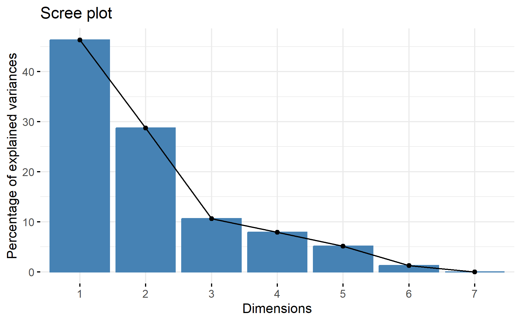
To explore the number of factors that could be determined different approaches are available. First, it is possible to apply PCA and evaluate the variability explained for each component. Thus, the table with the PCA results is shown below:
| PC1 | PC2 | PC3 | PC4 | PC5 | PC6 | PC7 | PC8 | PC9 | PC10 | PC11 | PC12 | PC13 | PC14 | PC15 | |
|---|---|---|---|---|---|---|---|---|---|---|---|---|---|---|---|
| Standard deviation | 2.2396 | 1.8402 | 1.2981 | 1.1391 | 0.9796 | 0.8921 | 0.7367 | 0.6430 | 0.5615 | 0.4988 | 0.3443 | 0.2865 | 0.2763 | 0.1809 | 0.1717 |
| Proportion of Variance | 0.3344 | 0.2258 | 0.1123 | 0.0865 | 0.0640 | 0.0531 | 0.0362 | 0.0276 | 0.0210 | 0.0166 | 0.0079 | 0.0055 | 0.0051 | 0.0022 | 0.0020 |
| Cumulative Proportion | 0.3344 | 0.5601 | 0.6725 | 0.7590 | 0.8230 | 0.8760 | 0.9122 | 0.9398 | 0.9608 | 0.9774 | 0.9853 | 0.9908 | 0.9958 | 0.9980 | 1.0000 |
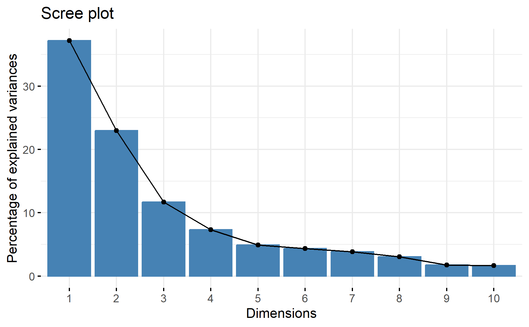
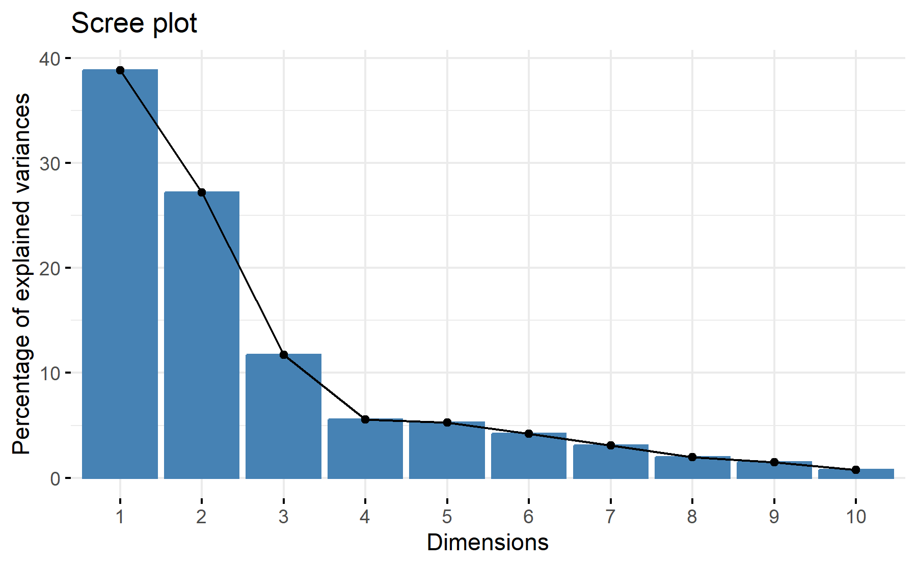
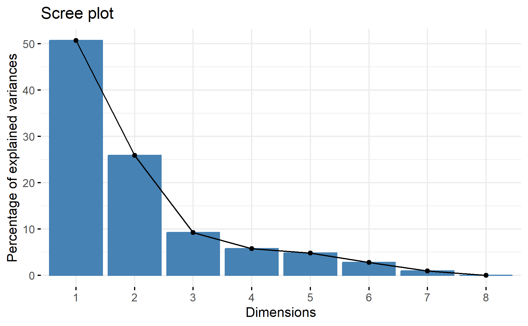
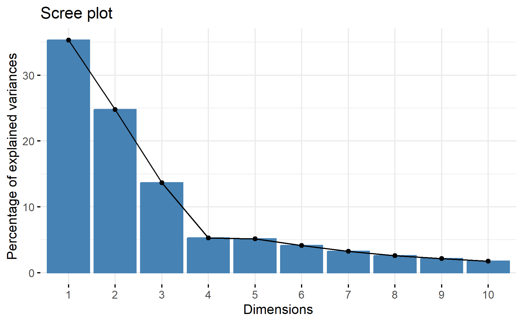
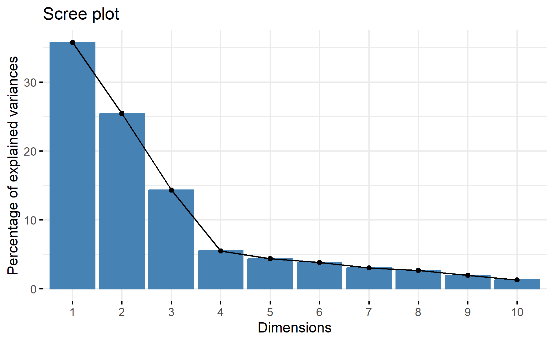
Then, the scree plot for this PCA analysis is displayed.
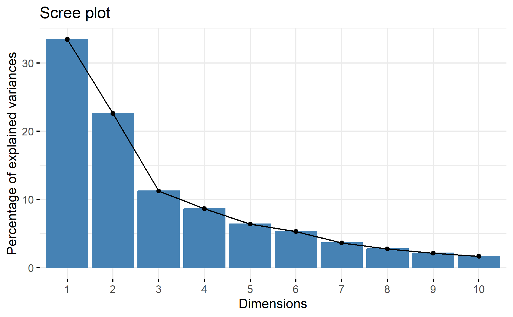 According to these results, 3 factors could be the best numbers. The cumulative proportion showed that with 3 components 67% of the variance could be explained, besides, just a 9% increase was added with an additional component. While the scree plot exhibit an elbow at the third component.
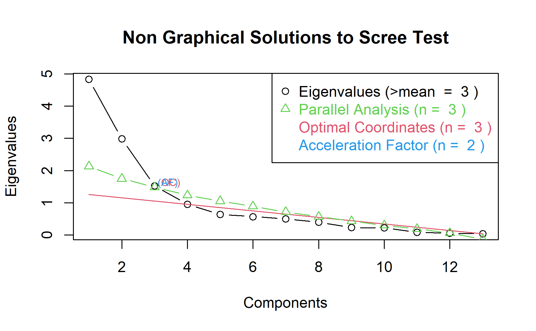
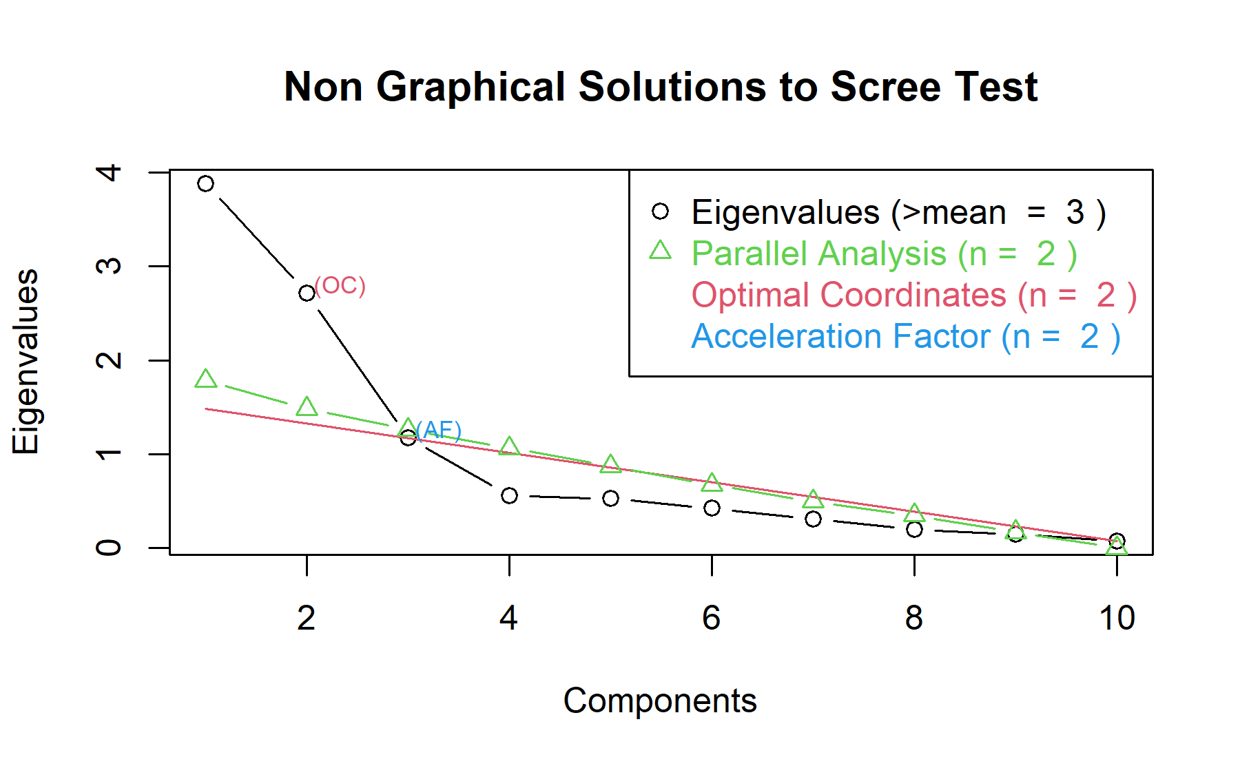
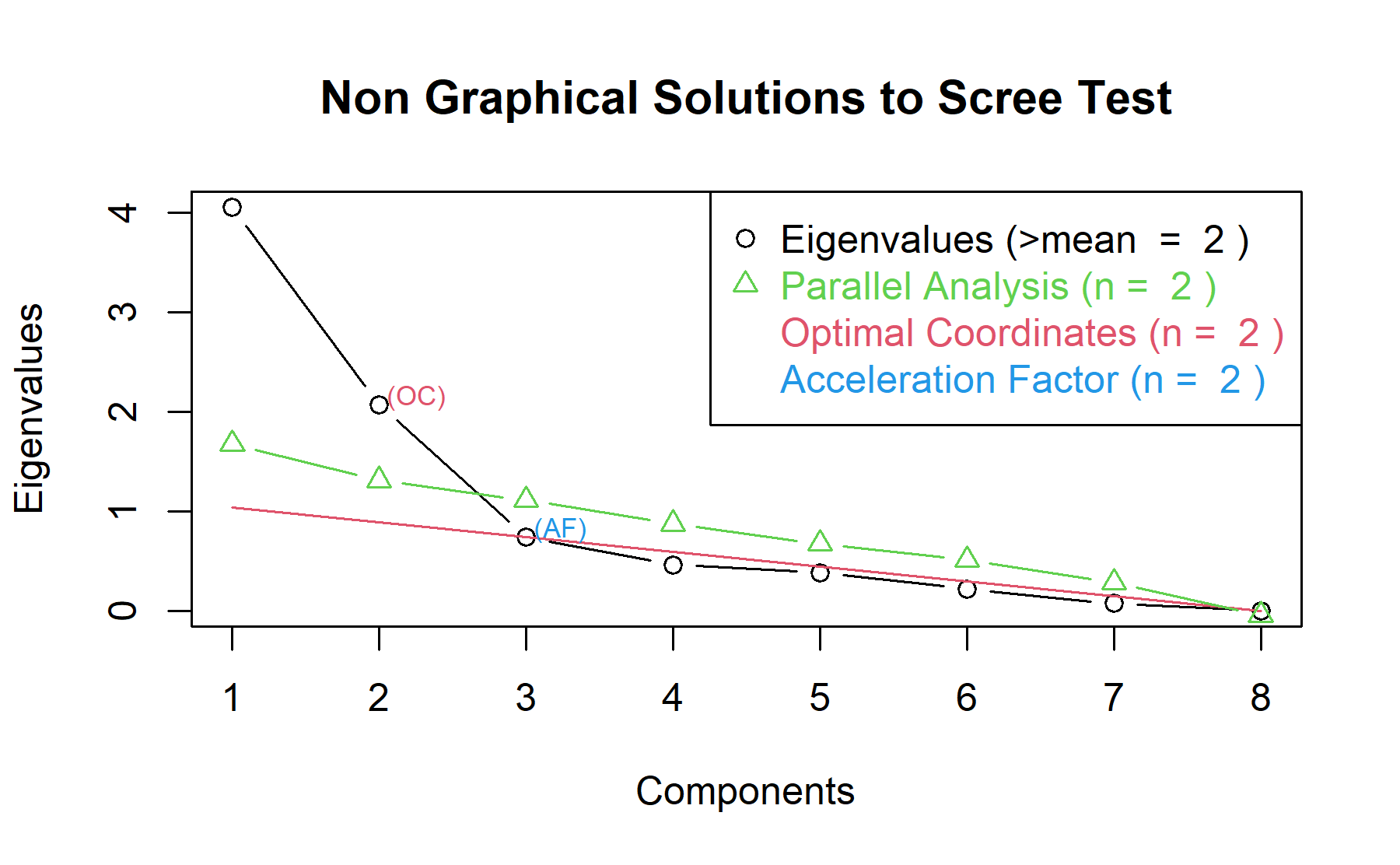
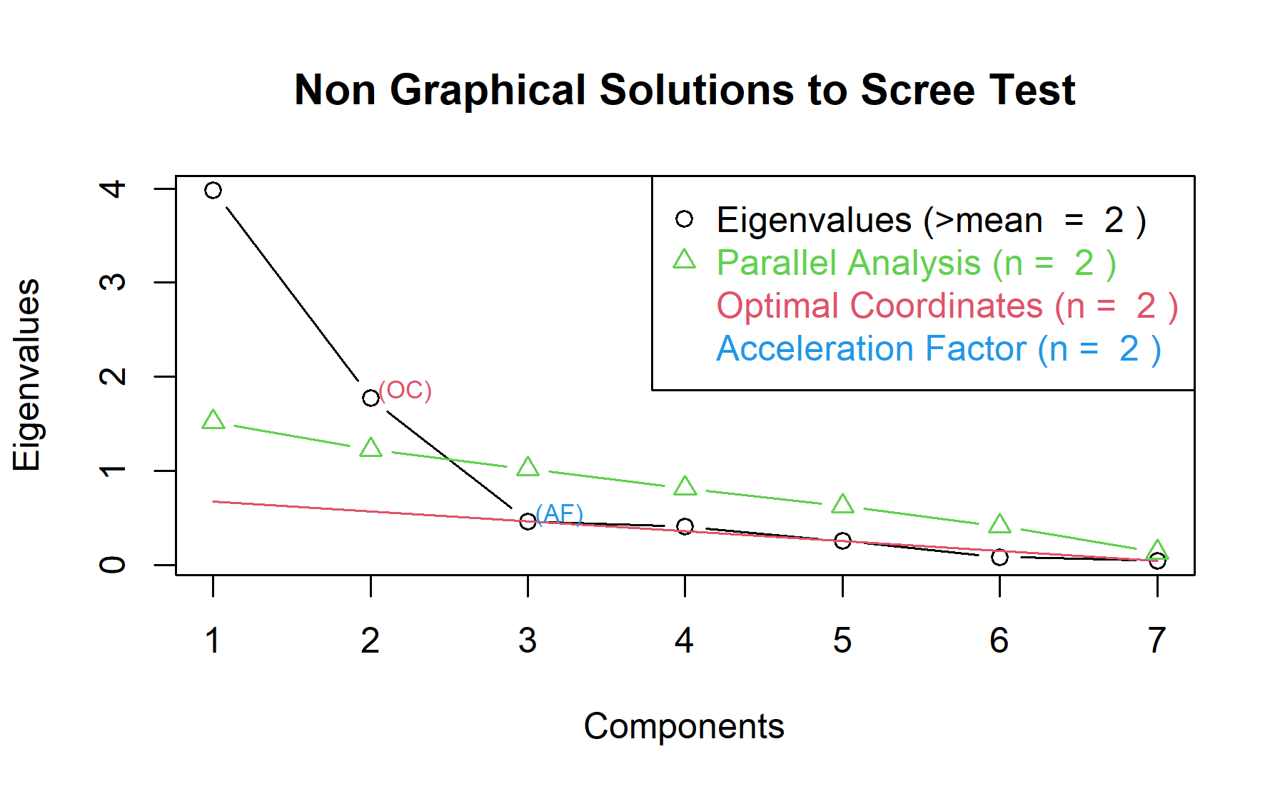
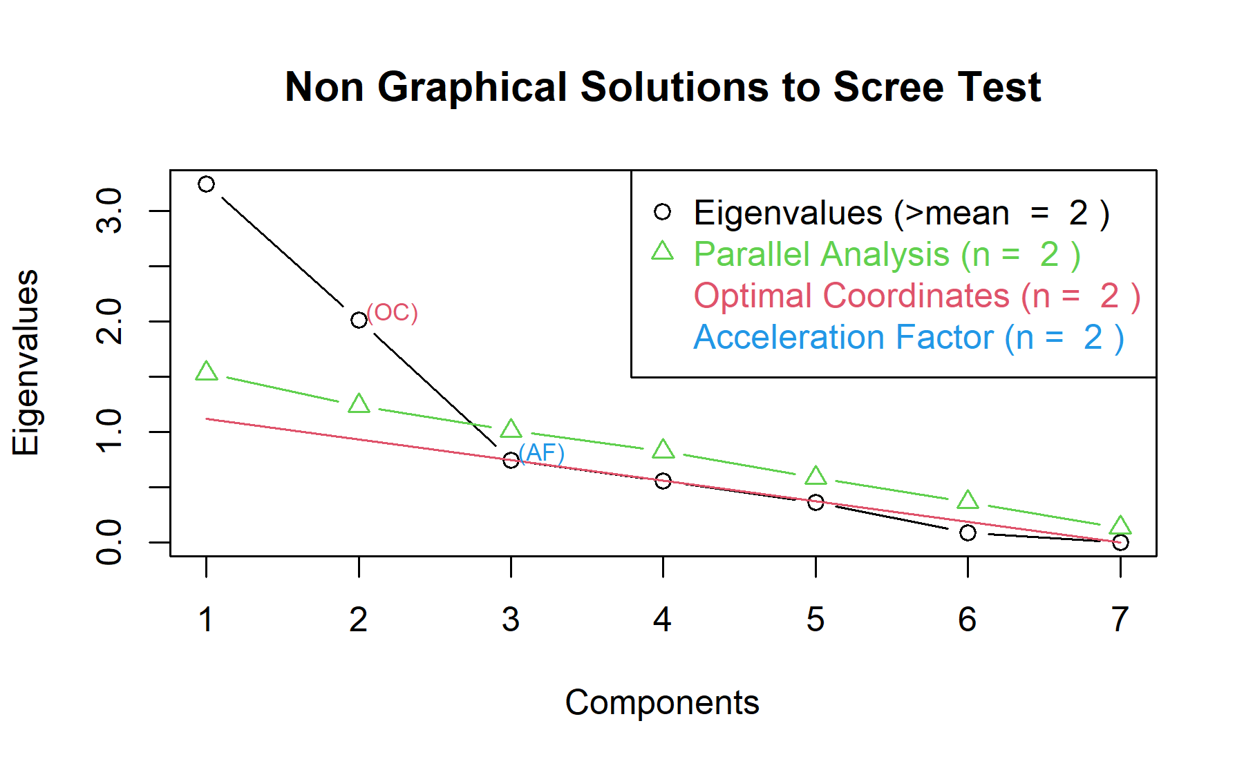
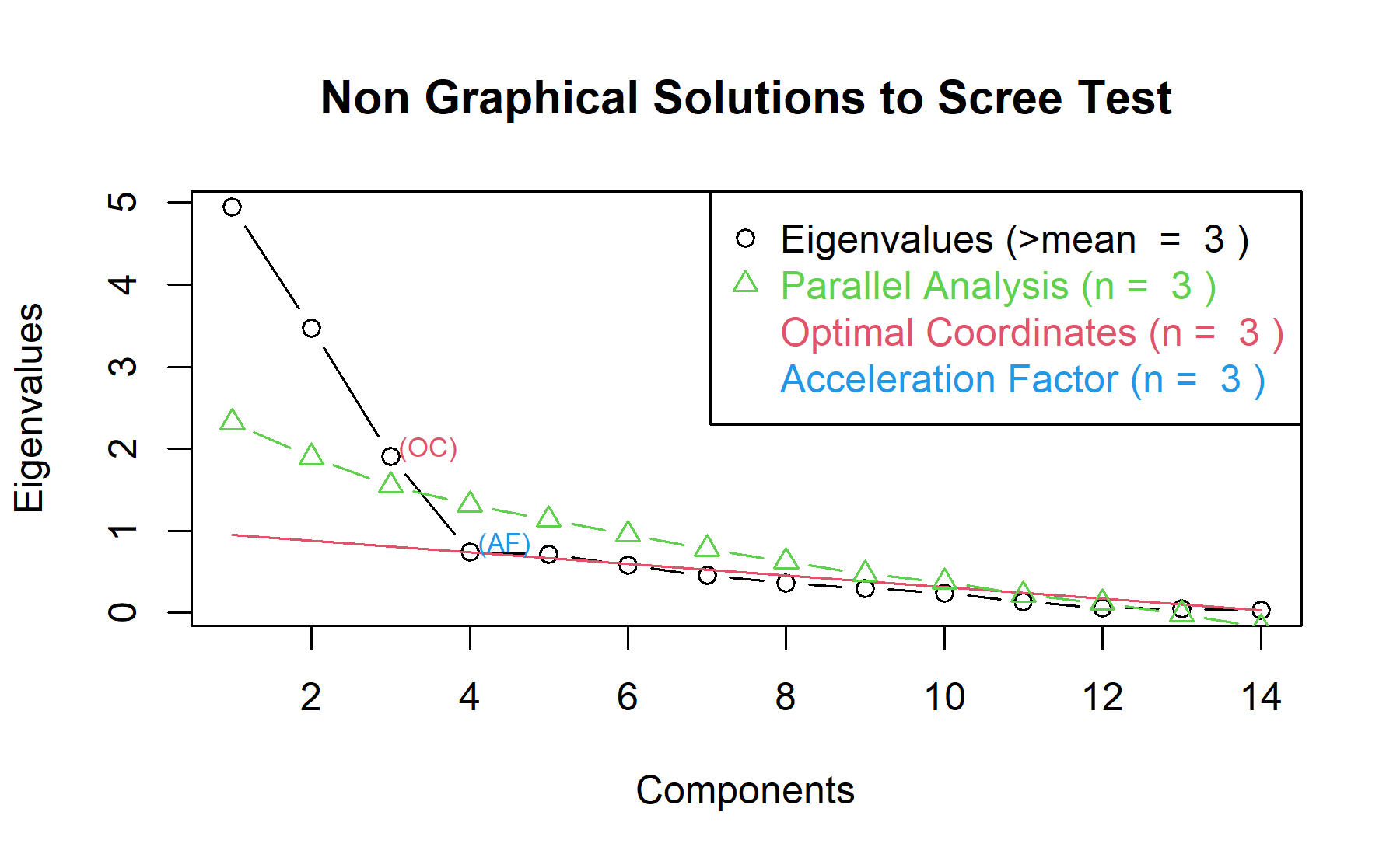
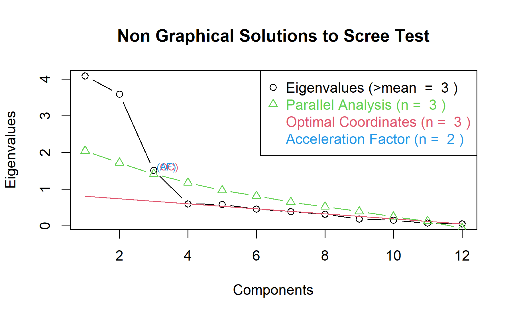
Then, another approach is implemented. With this strategy several analysis are combined and depict in the same figure. The tools implemented are: the Kaiser rule (which drops the components with eigenvalues < 1), the parallel analysis, and the usual scree test (plotuScree), the acceleration factor (which indicates where the elbow of the scree plot appears).
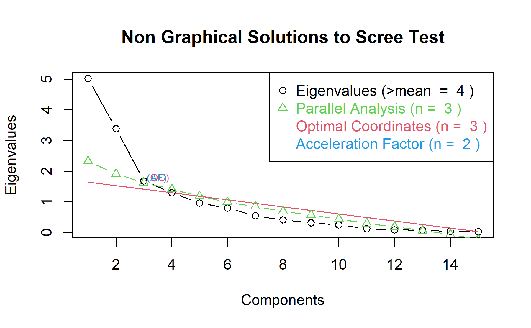 The acceleration factor chooses the number of factors before the elbow, which was found at the third component. The first criterion is defined according to the absolute value of the eigenvalues, with the criteria of choosing the ones below a threshold (1 or here the mean). In this setting, with this criterion 4 factors are suggested as the best combination. However, the other two criteria found 3 as the best number, similarly to what was identified in the prior analysis.
Initially, three factors will be considered.
Running the factor analysis with all the items (n=15), first the communalities are explored:
## Warning in cor.smooth(mat): Matrix was not positive definite, smoothing was
## done
## In smc, smcs < 0 were set to .0
## In smc, smcs < 0 were set to .0## In factor.stats, I could not find the RMSEA upper bound . Sorry about that## pre_exp_preoc_q1 pre_exp_preoc_q2 pre_exp_preoc_q3
## 0.3397 0.6007 0.3557
## pre_exp_preoc_q5 pre_exp_preoc_q6 pre_exp_preoc_q7_i
## 0.8704 0.9569 0.9950
## pre_exp_preoc_q7_ii pre_exp_preoc_q7_iii pre_exp_preoc_q7_iv
## 0.5992 0.7423 0.9619
## pre_exp_preoc_q7_v pre_exp_preoc_q8 pre_exp_preoc_q9
## 0.6863 0.7485 0.6234
## pre_exp_preoc_q10 pre_exp_preoc_q11 pre_exp_preoc_q4_Inverted
## 0.8103 0.7248 0.3524The communalities are the amount of the common variance for each item that can be explained by the factors. Thus, it is desirable to cover a considerable proportion of the it. To note, there is always an amount of variance (the unique variance) that is not explained by factors (a difference with the classical Principal Component Analysis in which all the variance is the common variance and can be explain by the principal components).
Therefore, considering the values of the communalities, again, Q1, Q3, and Q4 inv are those with lower values (<0.4)
Then, the whole output is displayed.
## Factor Analysis using method = ml
## Call: fa(r = pre_test_Q_ExpConcern_facAn, nfactors = 3, rotate = "oblimin",
## fm = "ml", cor = "poly")
## Standardized loadings (pattern matrix) based upon correlation matrix
## ML3 ML2 ML1 h2 u2 com
## pre_exp_preoc_q1 0.58 0.34 0.659 1.2
## pre_exp_preoc_q2 0.56 0.60 0.399 2.2
## pre_exp_preoc_q3 0.59 0.36 0.644 1.1
## pre_exp_preoc_q5 0.84 0.87 0.129 1.3
## pre_exp_preoc_q6 1.01 0.96 0.043 1.0
## pre_exp_preoc_q7_i 1.01 1.00 0.005 1.0
## pre_exp_preoc_q7_ii 0.75 0.60 0.401 1.0
## pre_exp_preoc_q7_iii 0.48 0.52 0.74 0.258 2.3
## pre_exp_preoc_q7_iv 0.82 0.96 0.038 1.4
## pre_exp_preoc_q7_v 0.64 0.69 0.314 1.6
## pre_exp_preoc_q8 0.85 0.75 0.251 1.2
## pre_exp_preoc_q9 0.74 0.62 0.376 1.1
## pre_exp_preoc_q10 0.89 0.81 0.190 1.1
## pre_exp_preoc_q11 0.83 0.73 0.275 1.0
## pre_exp_preoc_q4_Inverted -0.45 0.35 0.652 2.3
##
## ML3 ML2 ML1
## SS loadings 3.66 3.59 3.12
## Proportion Var 0.24 0.24 0.21
## Cumulative Var 0.24 0.48 0.69
## Proportion Explained 0.35 0.35 0.30
## Cumulative Proportion 0.35 0.70 1.00
##
## With factor correlations of
## ML3 ML2 ML1
## ML3 1.00 0.20 0.01
## ML2 0.20 1.00 0.42
## ML1 0.01 0.42 1.00
##
## Mean item complexity = 1.4
## Test of the hypothesis that 3 factors are sufficient.
##
## df null model = 105 with the objective function = 118.5 with Chi Square = 2034
## df of the model are 63 and the objective function was 105.7
##
## The root mean square of the residuals (RMSR) is 0.1
## The df corrected root mean square of the residuals is 0.13
##
## The harmonic n.obs is 24 with the empirical chi square 49.27 with prob < 0.9
## The total n.obs was 24 with Likelihood Chi Square = 1603 with prob < 2.7e-293
##
## Tucker Lewis Index of factoring reliability = -0.517
## RMSEA index = 1.008 and the 90 % confidence intervals are 0.987 NA
## BIC = 1402
## Fit based upon off diagonal values = 0.95
## Measures of factor score adequacy
## ML3 ML2 ML1
## Correlation of (regression) scores with factors 0.97 0.99 1.00
## Multiple R square of scores with factors 0.94 0.98 1.00
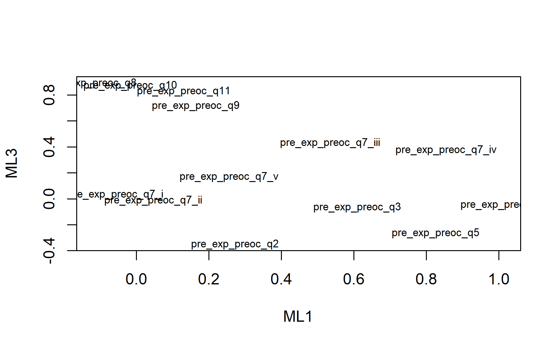
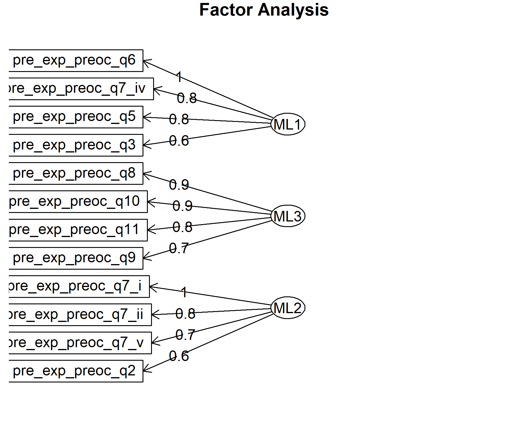
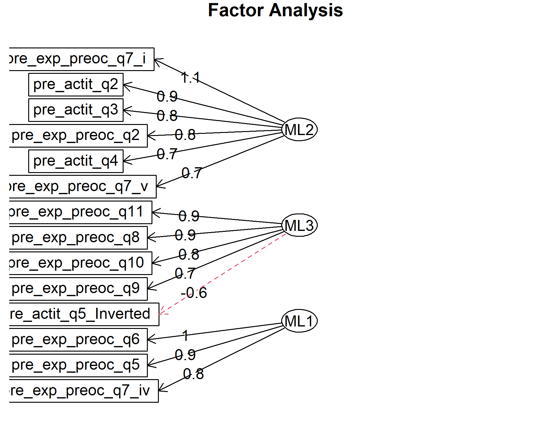
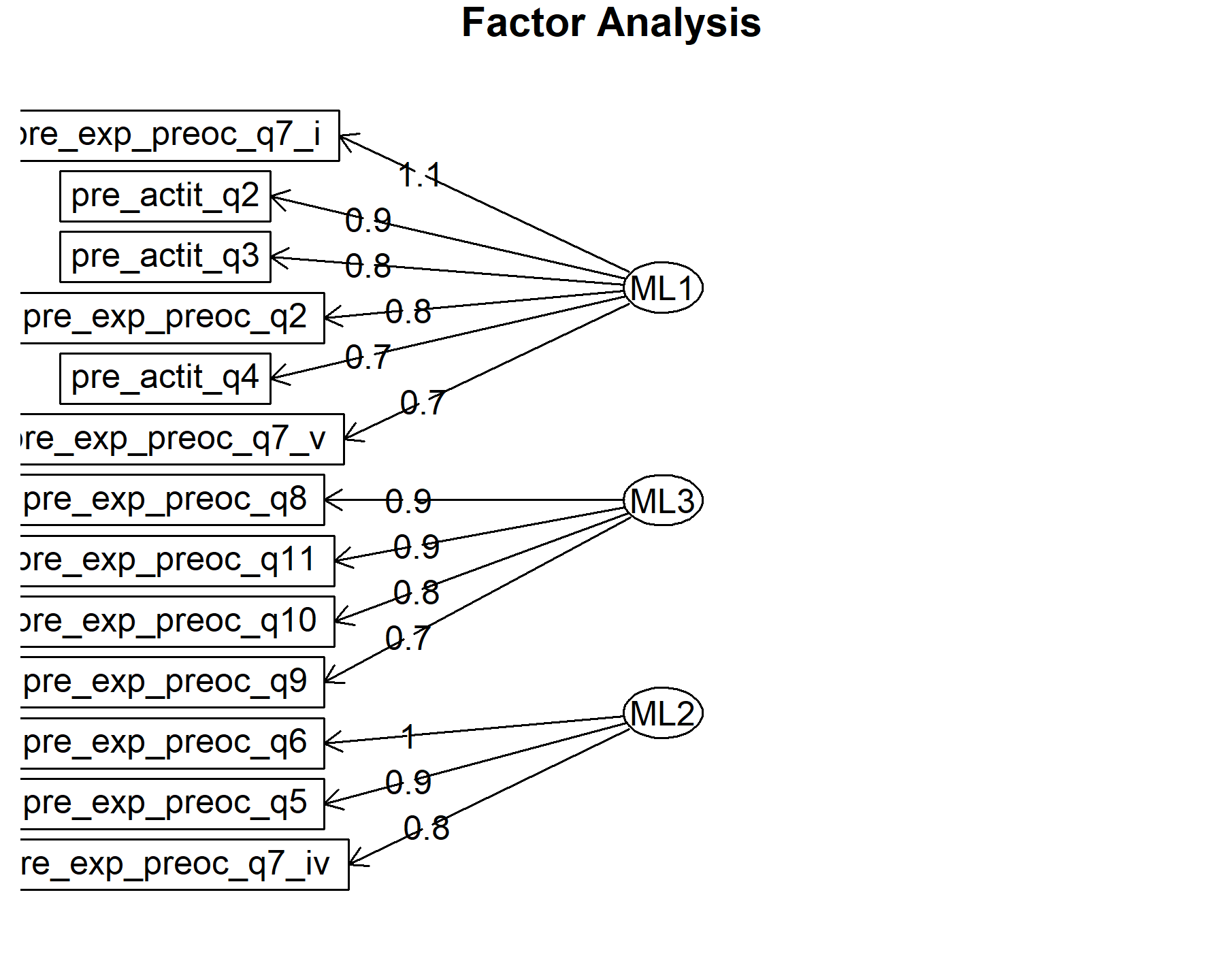
## Minimum correlation of possible factor scores 0.88 0.96 0.99Exploring these results, there are three factors composed by:
* Q1, Q2, Q7.i, Q7.ii, and Q7.v.
* Q3, Q5, Q6, and Q7.iv.
* Q8, Q9, Q10, Q11, and Q4 inv.
Q7.iii is linked with two factors. Besides, the association between Q4 inv and the ML3 is just above the threshold (with a low communality as well). It is important to highlight that Q7.iii (“Mi doctor cambiará mi tratamiento inmediatamente de acuerdo a los resultados.”) was mentioned before as a complex item, since this could be different for different patients. For some that will be true, while for others receiving a treatment the genomic testing is just to have additional information for the future. According to that, it is possible to find different relationships for this item to others depending on each subgroup of patients.
On the other hand, Q3 could be associated with Q5 and Q6 perhaps because the same patients having expectations about treatment options are the same that want to learn more.
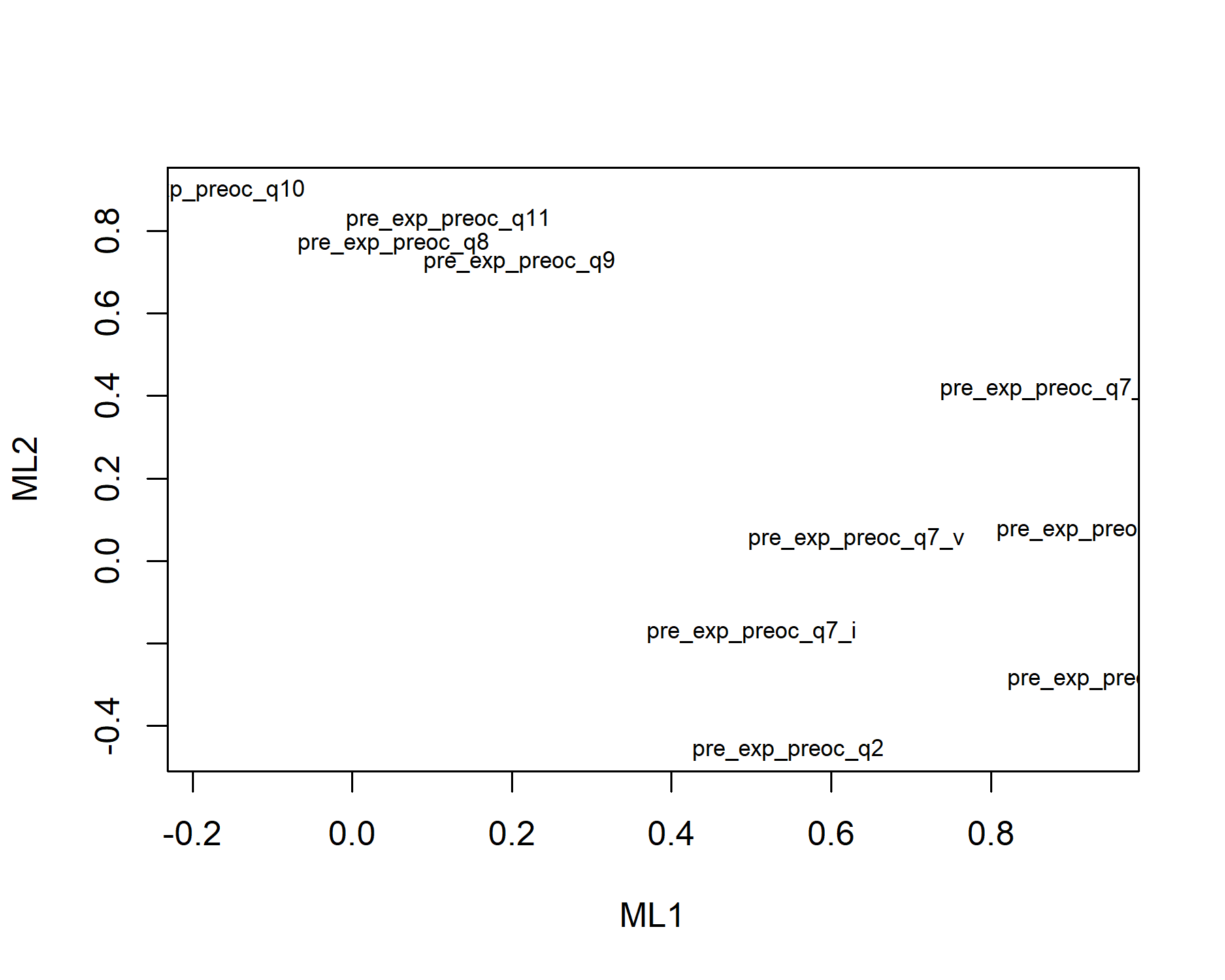
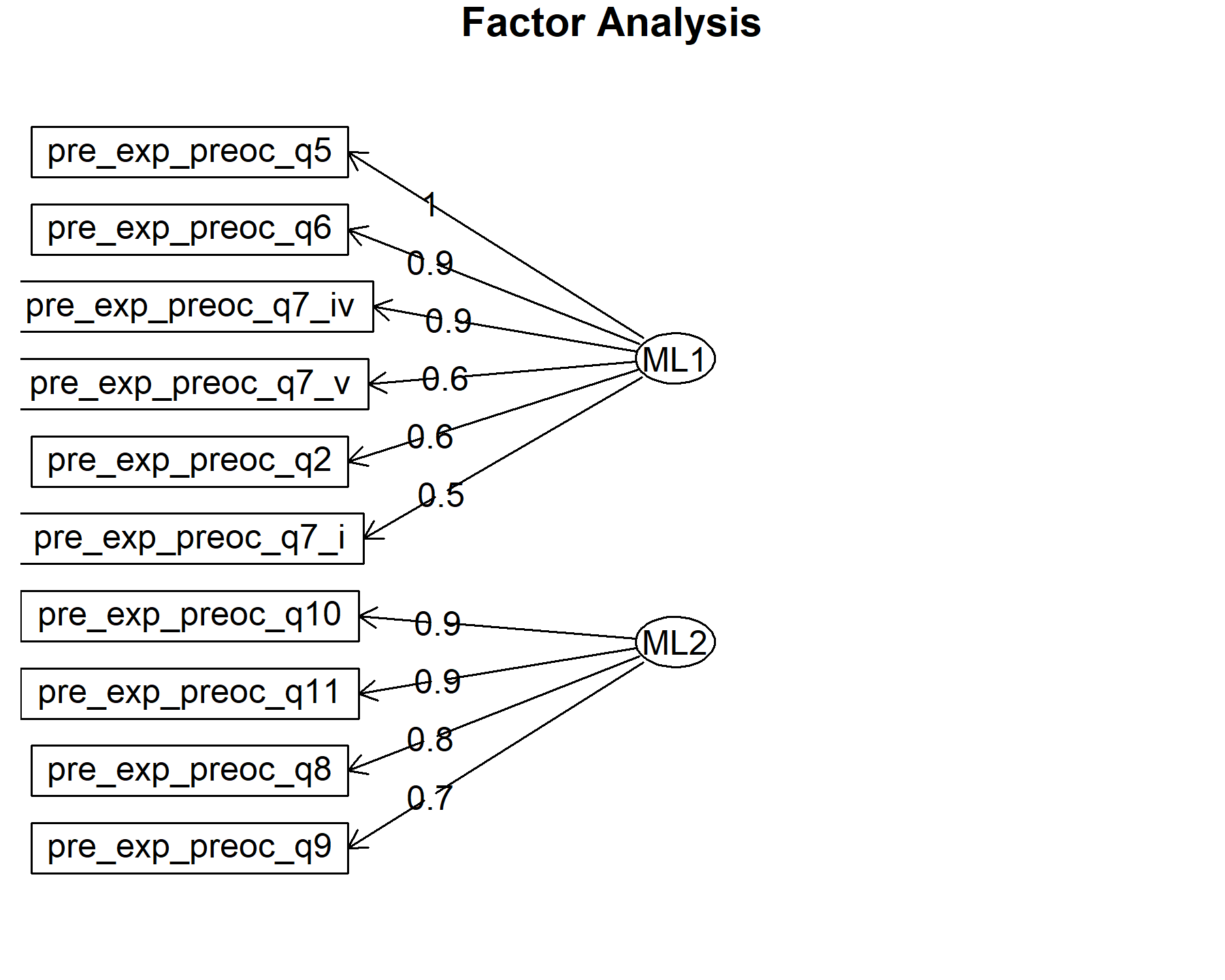
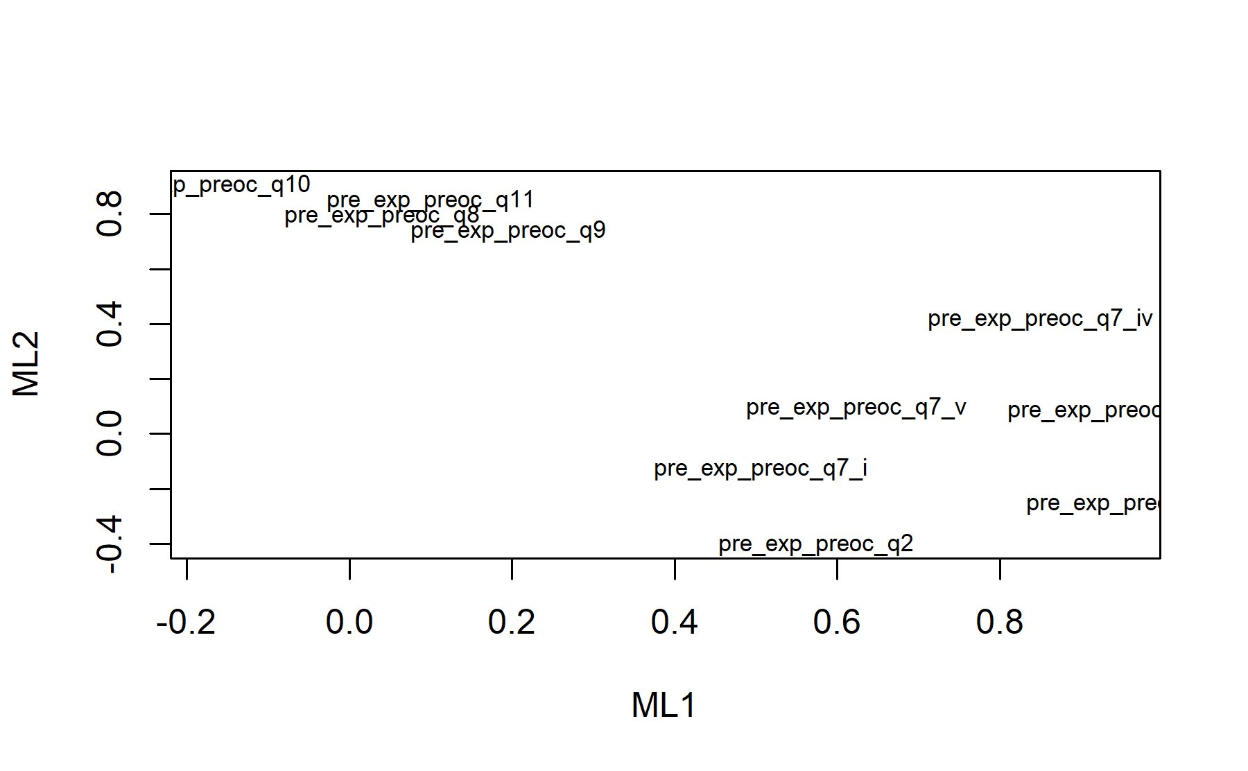
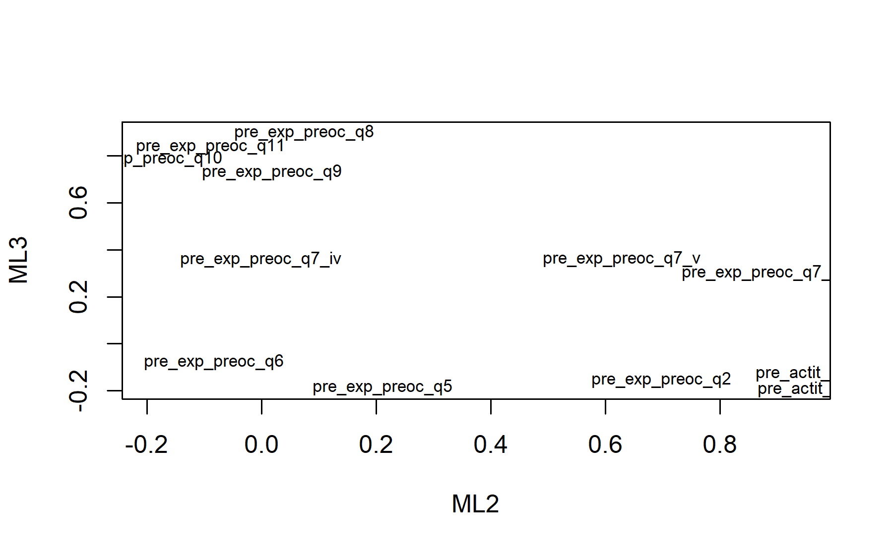
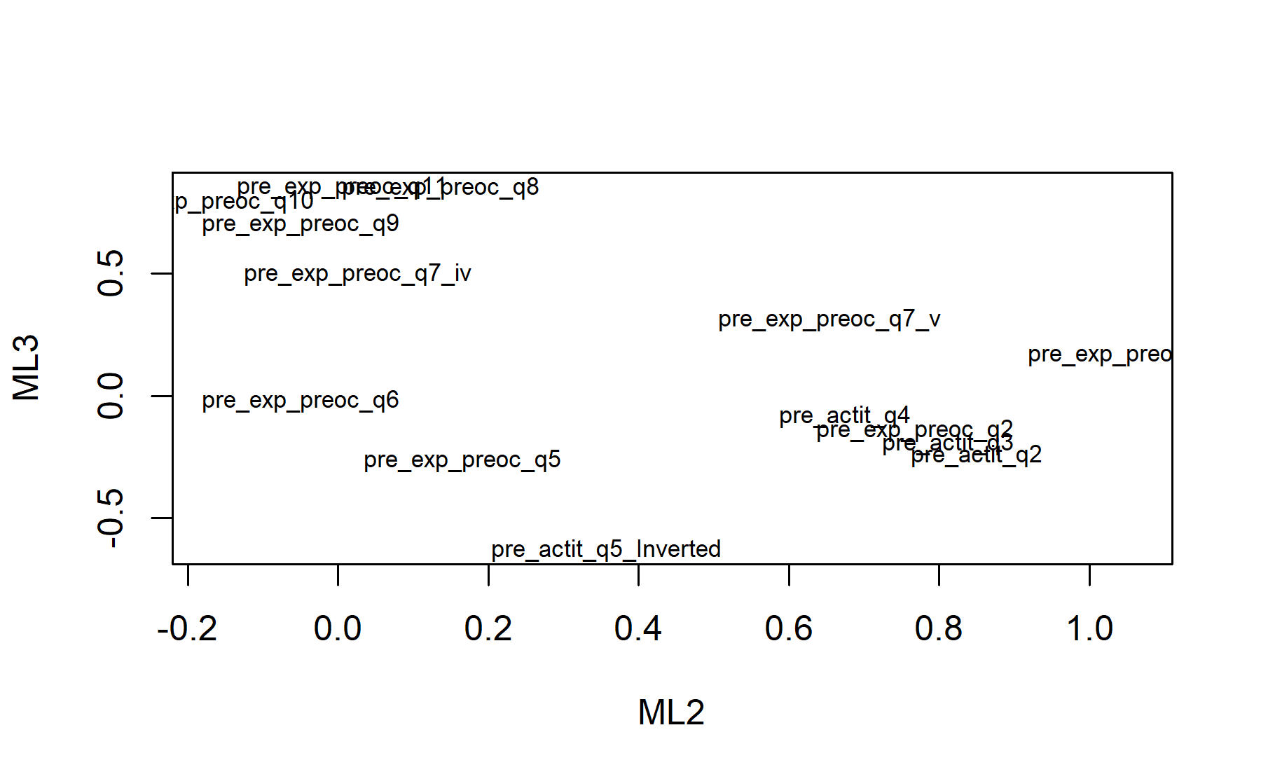
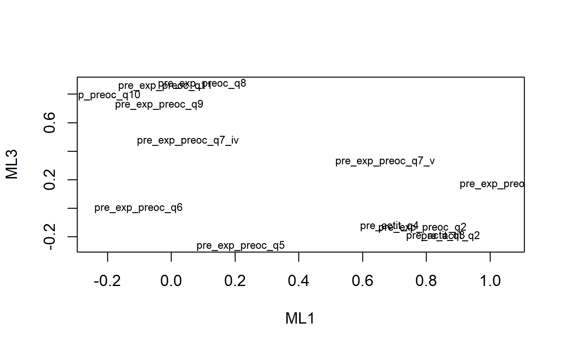
Finally, plots show the relationship between the items and the factors.
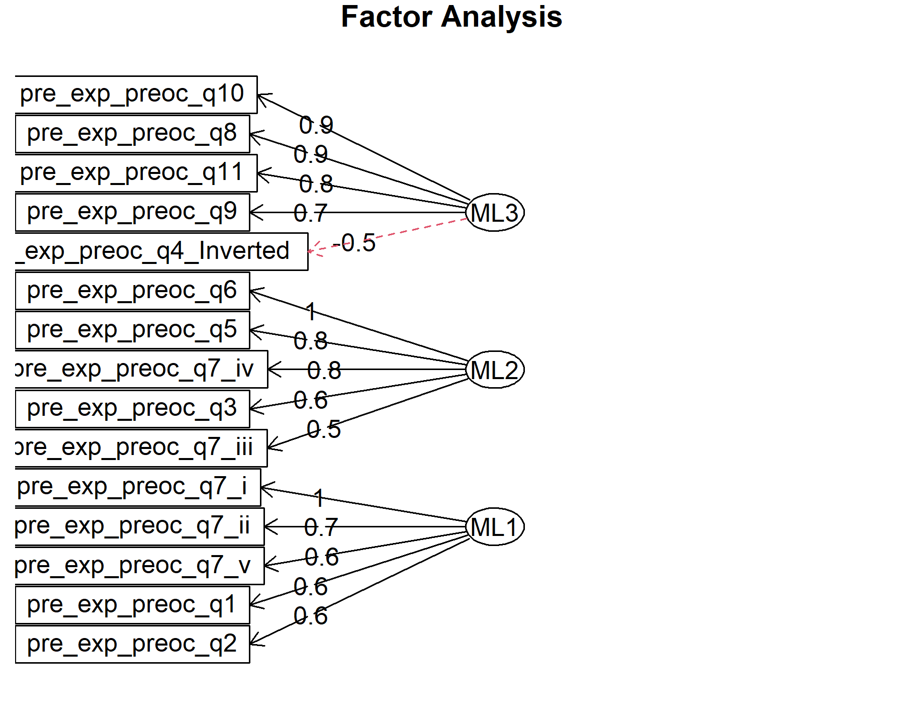
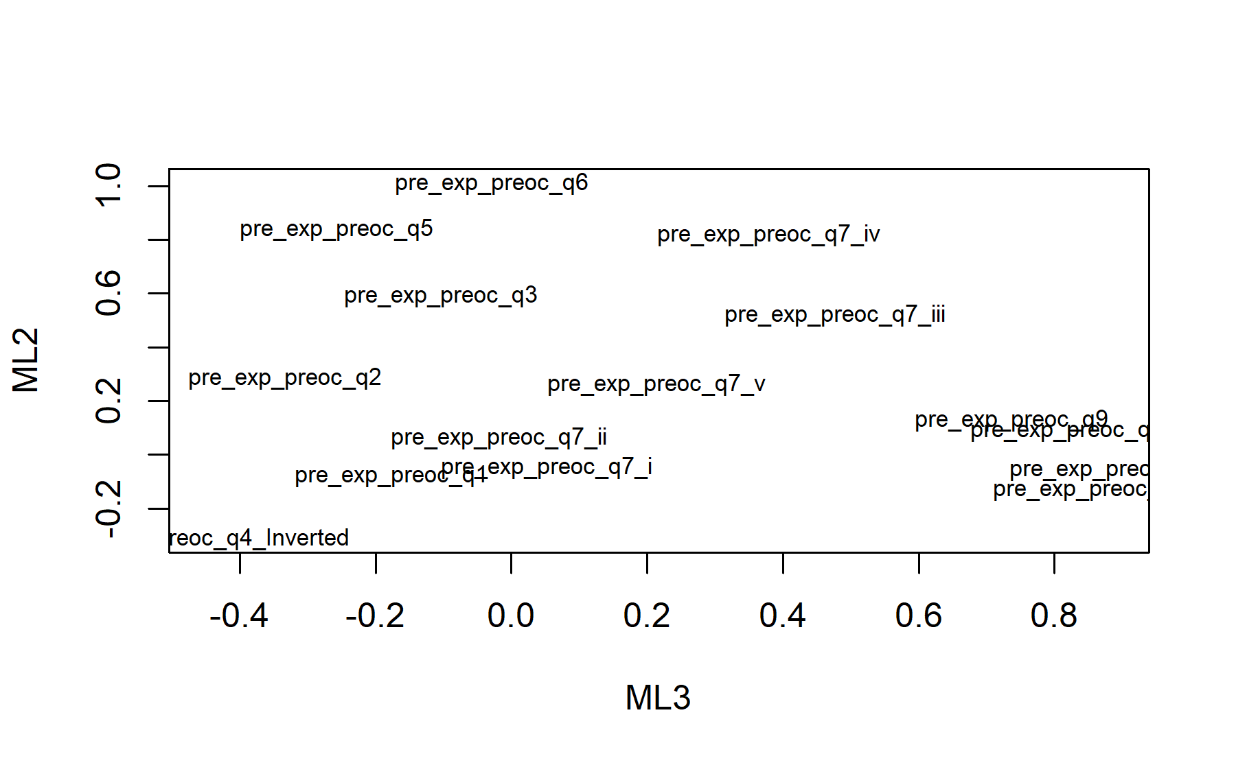
As first approach, the factor analysis is done with all the variables in order to have an exploratory view of the relationship between all the variables and the three factors. In this setting, all the variables are associated with only one factor except item 4-inverted.
These three factors are principally associated with the spheres and concepts previously described:
- Expectations of genomic results on treatment impact: item 5, 6, 7.iv, 7.v., and 7.iii.
- Expectations of results communications and the information provided: item 1, 2, 3, 4, 7.i, and 7.ii.
- Concerns: items 8, 9, 10, and 11.
Hence, the first factor is linked with the information concept; nevertheless, it does not include items 3 and 4, and has the item 7.v from treatment sphere. Q7.v ask about experimental therapies and perhaps those focused on that or looking for experimental options or clinical trials have certain information pattern. Then, the second factor is related with treatment impact; however, it includes item 3. Finally, the last factor includes all the concerns items plus Q4 inv.
Now, the same analysis is performed excluding the items previously identify as candidates to be left out.
- From descriptive and reliability analysis.
Potential items to be excluded according to the two expectations’ spheres:
- Expectations of genomic results on treatment impact: 7.iii, followed by 7.iv and 7.v. These two last items have adequate values, but they are the less critical ones in this sphere. Item 7.iv has a lower discrimination score than 7.v.
- Expectations of results communications and the information provided: 1 (if item 2 is selected), 4 due to its conflicting results along the analysis. Then item 3 and 7.ii showed conflicting results too. However, item 3 could be relevant if an interventional approach is considered.
With regard to the concerns domain, the there is not a clear difference between them. At least, item 11 seem to be relevant. The second item to be chosen can be identify when the rest of the analysis were completed.
From current factor analysis.
Considering the KMO, Q1, Q3, Q7_i, and Q4_Inv are under the threshold of 0.5.
Moreover, Q1, Q3, and Q4 inv have lower communalities. Then, Q7.iii was found related with two factors.Considering all together.
Therefore, as first approach Q1 and Q4 are the items identified in both, the first analysis and the factor analysis. Then other items, such as Q3 and Q7.iii, could be evaluated.
6.1.2 Excluding item 1 and 4.
Now, a new analysis is done considering all except Q1 and Q4.
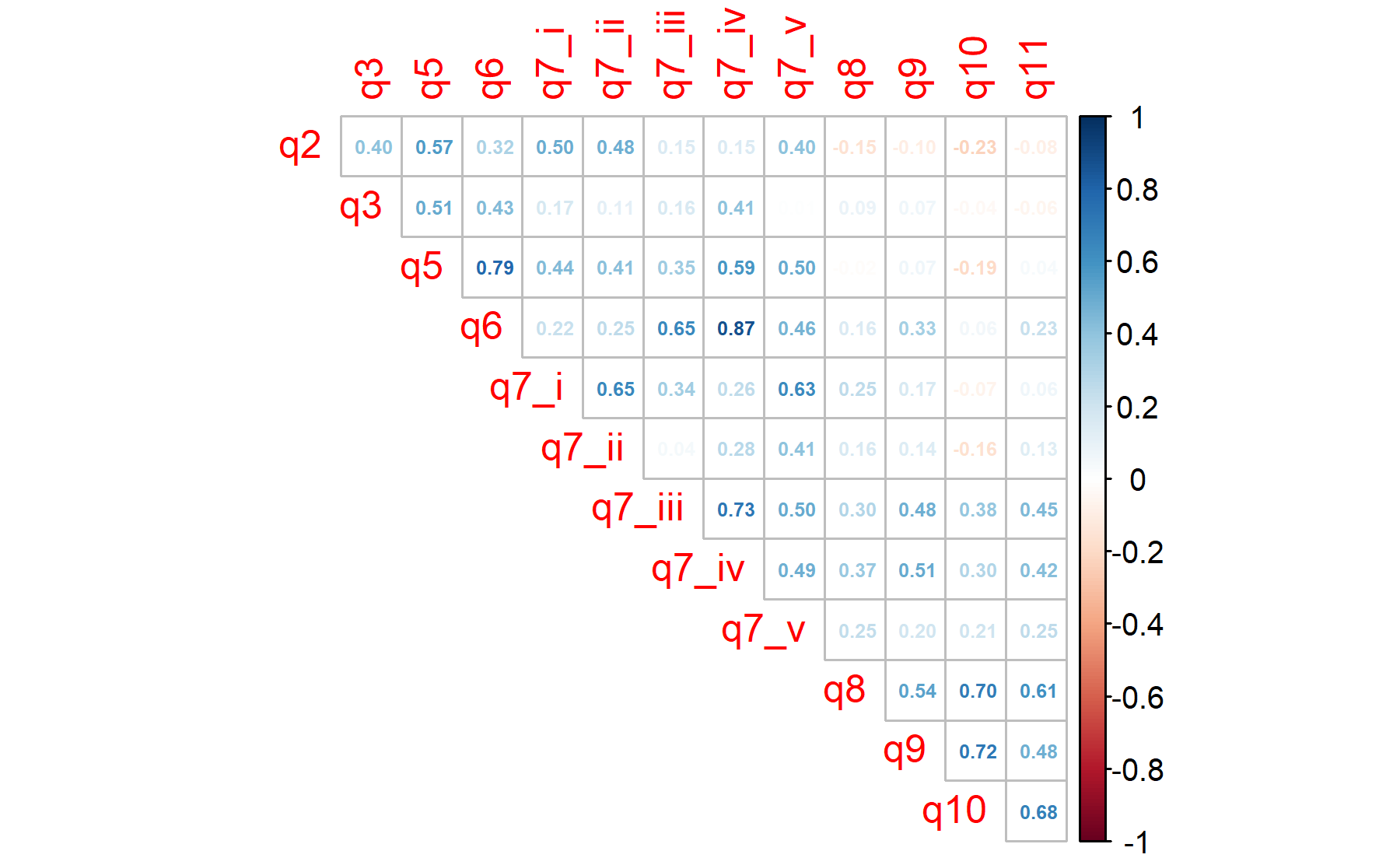
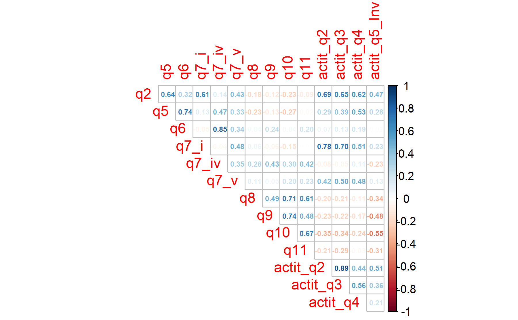
Figure 6.2: The list of the items are: 2.He recibido suficiente información para comprender beneficios y riesgos del análisis genómico, 3.Estoy interesado/a en aprender más, 5.El resultado ayudará al control de mi cáncer, 6.El resultado ayudará a aumentar mi expectativa vida, 7i.Mi Dr me explicará resultados y la implicación para mi salud, 7ii.Recibiré informe escrito con el resultado, 7iii.Mi Dr cambiará mi tto de acuerdo a los resultados, 7iv.Tendré opciones de tratamiento adicionales, 7v.Podré recibir tratamientos experimentales, 8.Me preocupa que los resultados puedan no guiar mi tratamiento, 9.Me preocupa que los resultados pueden ser difíciles de comprender, 10.Me preocupa que los resultados pueden dar información del riesgo de enf que preferiría no saber, 11.Los resultados pueden preocuparme o generar ansiedad
The Barlett’s sphericity test is performed.
Thus, the p-value = 0 and the H0 is rejected confirming the utility of applying a factor analysis to this dataset.
## Kaiser-Meyer-Olkin factor adequacy
## Call: KMO(r = pre_test_Q_ExpConcern_facAn_2_corr)
## Overall MSA =  0.59
## MSA for each item =
##     q2     q3     q5     q6   q7_i  q7_ii q7_iii  q7_iv   q7_v     q8     q9
##   0.67   0.42   0.71   0.64   0.44   0.56   0.61   0.72   0.54   0.58   0.54
##    q10    q11
##   0.48   0.70
To explore the number of factors the same approach is conducted. Thus, the table with the PCA results is shown below:
| PC1 | PC2 | PC3 | PC4 | PC5 | PC6 | PC7 | PC8 | PC9 | PC10 | PC11 | PC12 | PC13 | |
|---|---|---|---|---|---|---|---|---|---|---|---|---|---|
| Standard deviation | 2.1985 | 1.7278 | 1.2335 | 0.9751 | 0.7983 | 0.7524 | 0.7071 | 0.6274 | 0.4759 | 0.4660 | 0.2850 | 0.2244 | 0.1919 |
| Proportion of Variance | 0.3718 | 0.2296 | 0.1170 | 0.0731 | 0.0490 | 0.0436 | 0.0385 | 0.0303 | 0.0174 | 0.0167 | 0.0063 | 0.0039 | 0.0028 |
| Cumulative Proportion | 0.3718 | 0.6014 | 0.7185 | 0.7916 | 0.8406 | 0.8842 | 0.9226 | 0.9529 | 0.9703 | 0.9870 | 0.9933 | 0.9972 | 1.0000 |
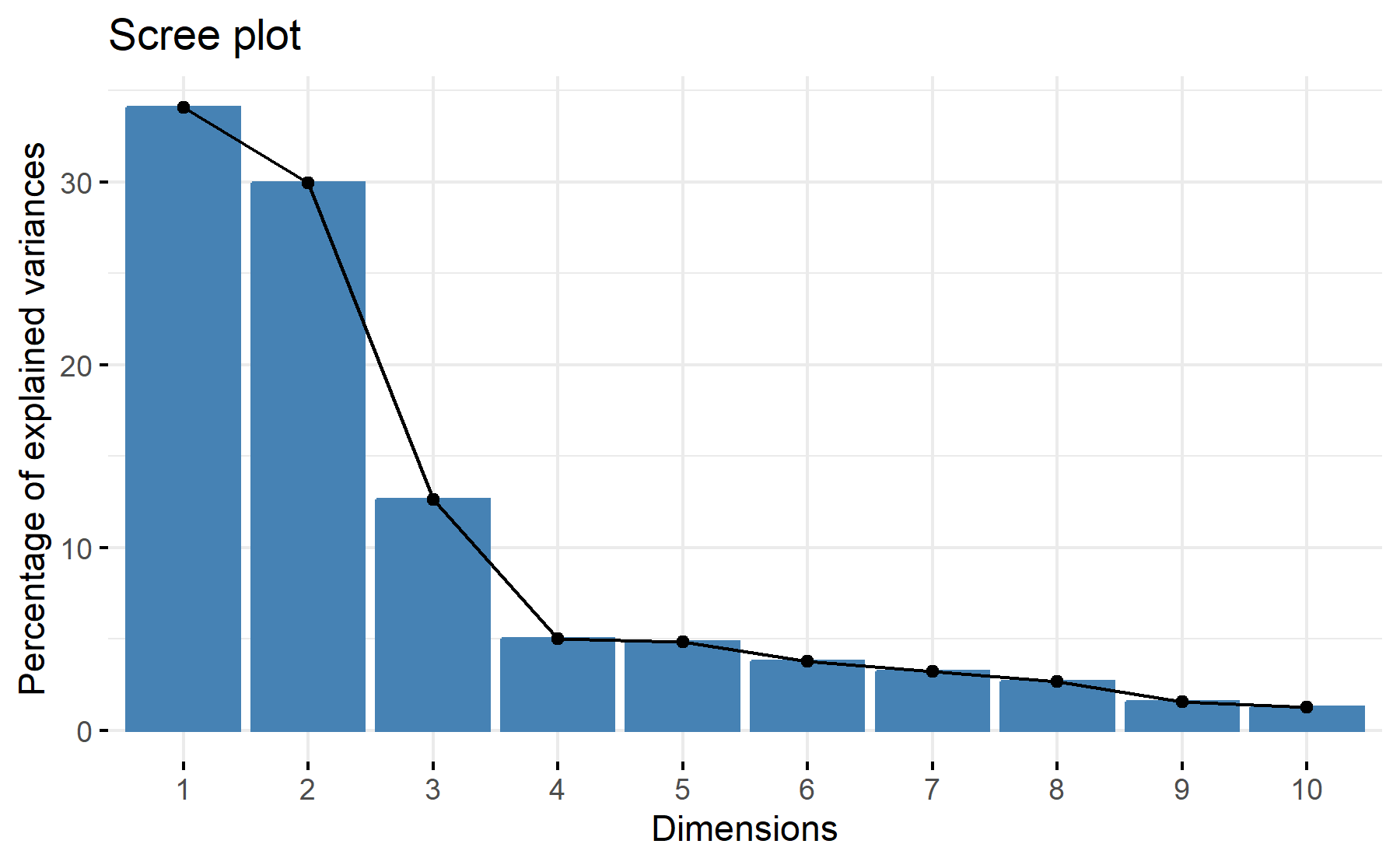
Then, the scree plot for this PCA analysis is displayed.
 According to these results, 3 factors could be the best numbers. The cumulative proportion showed that with 3 components 72% of the variance could be explained, besides, just a 7% increase was added with an additional component. The scree plot exhibit two steps, in the second and the third component, with then an elbow at the third-four component.
Then, another approach is implemented. With this strategy several analysis are combined and depict in the same figure. The tools implemented are: the Kaiser rule (which drops the components with eigenvalues < 1), the parallel analysis, and the usual scree test (plotuScree), the acceleration factor (which indicates where the elbow of the scree plot appears).
With this approach two factors are suggested as the best strategy. Thus, both approaches will be studied considering two and three factors.
## Warning in cor.smooth(mat): Matrix was not positive definite, smoothing was
## done
## In factor.stats, I could not find the RMSEA upper bound . Sorry about that## pre_exp_preoc_q2 pre_exp_preoc_q3 pre_exp_preoc_q5
## 0.6099 0.3795 0.8780
## pre_exp_preoc_q6 pre_exp_preoc_q7_i pre_exp_preoc_q7_ii
## 0.9640 0.9950 0.6127
## pre_exp_preoc_q7_iii pre_exp_preoc_q7_iv pre_exp_preoc_q7_v
## 0.7048 0.9950 0.6709
## pre_exp_preoc_q8 pre_exp_preoc_q9 pre_exp_preoc_q10
## 0.8428 0.6074 0.7961
## pre_exp_preoc_q11
## 0.7393While most the items are well explained by the factors, in line with previous findings, Q3 still has a low communality result.
## Factor Analysis using method =  ml
## Call: fa(r = pre_test_Q_ExpConcern_facAn_2, nfactors = 3, rotate = "oblimin",
##     fm = "ml", cor = "poly")
## Standardized loadings (pattern matrix) based upon correlation matrix
##                        ML1   ML3   ML2   h2     u2 com
## pre_exp_preoc_q2                  0.57 0.61 0.3912 2.2
## pre_exp_preoc_q3      0.61             0.37 0.6255 1.0
## pre_exp_preoc_q5      0.83             0.88 0.1224 1.4
## pre_exp_preoc_q6      1.01             0.96 0.0360 1.0
## pre_exp_preoc_q7_i                1.02 1.00 0.0050 1.0
## pre_exp_preoc_q7_ii               0.76 0.61 0.3868 1.0
## pre_exp_preoc_q7_iii  0.53  0.43       0.70 0.2951 2.3
## pre_exp_preoc_q7_iv   0.85             1.00 0.0049 1.4
## pre_exp_preoc_q7_v                0.64 0.67 0.3285 1.5
## pre_exp_preoc_q8            0.89       0.84 0.1569 1.2
## pre_exp_preoc_q9            0.72       0.61 0.3931 1.1
## pre_exp_preoc_q10           0.87       0.80 0.2042 1.1
## pre_exp_preoc_q11           0.83       0.74 0.2613 1.1
##
##                        ML1  ML3  ML2
## SS loadings           3.58 3.38 2.83
## Proportion Var        0.28 0.26 0.22
## Cumulative Var        0.28 0.54 0.75
## Proportion Explained  0.37 0.34 0.29
## Cumulative Proportion 0.37 0.71 1.00
##
##  With factor correlations of
##      ML1  ML3  ML2
## ML1 1.00 0.18 0.43
## ML3 0.18 1.00 0.04
## ML2 0.43 0.04 1.00
##
## Mean item complexity =  1.3
## Test of the hypothesis that 3 factors are sufficient.
##
## df null model =  78  with the objective function =  76.25 with Chi Square =  1360
## df of  the model are 42  and the objective function was  63.28
##
## The root mean square of the residuals (RMSR) is  0.07
## The df corrected root mean square of the residuals is  0.1
##
## The harmonic n.obs is  24 with the empirical chi square  19.38  with prob <  1
## The total n.obs was  24  with Likelihood Chi Square =  1002  with prob <  1.2e-182
##
## Tucker Lewis Index of factoring reliability =  -0.579
## RMSEA index =  0.975  and the 90 % confidence intervals are  0.944 NA
## BIC =  868.4
## Fit based upon off diagonal values = 0.98
## Measures of factor score adequacy
##                                                    ML1  ML3  ML2
## Correlation of (regression) scores with factors   0.99 0.98 1.00
## Multiple R square of scores with factors          0.99 0.96 1.00
## Minimum correlation of possible factor scores     0.98 0.91 0.99
There are three factors composed by:
* Q3, Q5, Q6, and Q7.iv.
* Q8, Q9, Q10, and Q11.
* Q2, Q7.i, Q7.ii, and Q7.v.
Finally, plots show the relationship between the items and the factors.

The results now are more consistent. The only issue is the finding that item Q7.iii is still belonging to two items.
A last approach will be considered excluding this item.
6.1.3 Excluding item 1, 4, and 7.iii.
The Barlett’s sphericity test is performed.
Thus, the p-value = 0 and the H0 is rejected confirming the utility of applying a factor analysis to this dataset.
## Kaiser-Meyer-Olkin factor adequacy
## Call: KMO(r = pre_test_Q_ExpConcern_facAn_3_corr)
## Overall MSA =  0.58
## MSA for each item =
##    q2    q3    q5    q6  q7_i q7_ii q7_iv  q7_v    q8    q9   q10   q11
##  0.66  0.43  0.74  0.61  0.53  0.64  0.65  0.51  0.62  0.49  0.45  0.67
To explore the number of factors the same approach is conducted. Thus, the table with the PCA results is shown below:
| PC1 | PC2 | PC3 | PC4 | PC5 | PC6 | PC7 | PC8 | PC9 | PC10 | PC11 | PC12 | |
|---|---|---|---|---|---|---|---|---|---|---|---|---|
| Standard deviation | 2.0809 | 1.7154 | 1.2202 | 0.9222 | 0.7796 | 0.7383 | 0.7061 | 0.4865 | 0.4758 | 0.4203 | 0.2307 | 0.2081 |
| Proportion of Variance | 0.3608 | 0.2452 | 0.1241 | 0.0709 | 0.0506 | 0.0454 | 0.0415 | 0.0197 | 0.0189 | 0.0147 | 0.0044 | 0.0036 |
| Cumulative Proportion | 0.3608 | 0.6061 | 0.7302 | 0.8010 | 0.8517 | 0.8971 | 0.9386 | 0.9584 | 0.9772 | 0.9920 | 0.9964 | 1.0000 |
Then, the scree plot for this PCA analysis is displayed.
 According to these results, 3 factors could be the best numbers. The cumulative proportion showed that with 3 components 73% of the variance could be explained, besides, just a 7% increase was added with an additional component. The scree plot exhibit an elbow at the third component.
Then, another approach is implemented. With this strategy several analysis are combined and depict in the same figure. The tools implemented are: the Kaiser rule (which drops the components with eigenvalues < 1), the parallel analysis, and the usual scree test (plotuScree), the acceleration factor (which indicates where the elbow of the scree plot appears).

According to the analysis, three factors seems to be an adequate approach.
## Warning in cor.smooth(mat): Matrix was not positive definite, smoothing was
## done
## In factor.stats, I could not find the RMSEA upper bound . Sorry about that## pre_exp_preoc_q2 pre_exp_preoc_q3 pre_exp_preoc_q5 pre_exp_preoc_q6
## 0.6126 0.3707 0.9000 0.9730
## pre_exp_preoc_q7_i pre_exp_preoc_q7_ii pre_exp_preoc_q7_iv pre_exp_preoc_q7_v
## 0.9950 0.6978 0.9950 0.6947
## pre_exp_preoc_q8 pre_exp_preoc_q9 pre_exp_preoc_q10 pre_exp_preoc_q11
## 0.8573 0.5934 0.7752 0.7491While most the items are well explained by the factors, in line with previous findings, Q3 still has a low communality result.
## Factor Analysis using method =  ml
## Call: fa(r = pre_test_Q_ExpConcern_facAn_3, nfactors = 3, rotate = "oblimin",
##     fm = "ml", cor = "poly")
## Standardized loadings (pattern matrix) based upon correlation matrix
##                       ML1   ML3   ML2   h2     u2 com
## pre_exp_preoc_q2                 0.58 0.61 0.3855 2.1
## pre_exp_preoc_q3     0.59             0.37 0.6281 1.0
## pre_exp_preoc_q5     0.81             0.90 0.1002 1.4
## pre_exp_preoc_q6     1.01             0.97 0.0270 1.0
## pre_exp_preoc_q7_i               1.02 1.00 0.0049 1.0
## pre_exp_preoc_q7_ii              0.82 0.70 0.3012 1.0
## pre_exp_preoc_q7_iv  0.85             1.00 0.0049 1.4
## pre_exp_preoc_q7_v               0.66 0.69 0.3059 1.5
## pre_exp_preoc_q8           0.89       0.86 0.1422 1.3
## pre_exp_preoc_q9           0.71       0.59 0.4078 1.2
## pre_exp_preoc_q10          0.86       0.77 0.2256 1.1
## pre_exp_preoc_q11          0.84       0.75 0.2498 1.1
##
##                        ML1  ML3  ML2
## SS loadings           3.19 3.13 2.89
## Proportion Var        0.27 0.26 0.24
## Cumulative Var        0.27 0.53 0.77
## Proportion Explained  0.35 0.34 0.31
## Cumulative Proportion 0.35 0.69 1.00
##
##  With factor correlations of
##      ML1  ML3  ML2
## ML1 1.00 0.14 0.41
## ML3 0.14 1.00 0.01
## ML2 0.41 0.01 1.00
##
## Mean item complexity =  1.3
## Test of the hypothesis that 3 factors are sufficient.
##
## df null model =  66  with the objective function =  74.06 with Chi Square =  1345
## df of  the model are 33  and the objective function was  61.64
##
## The root mean square of the residuals (RMSR) is  0.07
## The df corrected root mean square of the residuals is  0.1
##
## The harmonic n.obs is  24 with the empirical chi square  15.81  with prob <  1
## The total n.obs was  24  with Likelihood Chi Square =  996.5  with prob <  5.3e-188
##
## Tucker Lewis Index of factoring reliability =  -0.703
## RMSEA index =  1.102  and the 90 % confidence intervals are  1.067 NA
## BIC =  891.6
## Fit based upon off diagonal values = 0.98
## Measures of factor score adequacy
##                                                    ML1  ML3  ML2
## Correlation of (regression) scores with factors   1.00 0.98 1.00
## Multiple R square of scores with factors          0.99 0.96 1.00
## Minimum correlation of possible factor scores     0.98 0.92 0.99
There are three factors composed by:
* Q3, Q5, Q6, and Q7.iv.
* Q8, Q9, Q10, and Q11.
* Q2, Q7.i, Q7.ii, and Q7.v.
Finally, plots show the relationship between the items and the factors.

6.1.4 Excluding items Q1, Q4, Q7_ii, Q7_iii and Q3.
The first two items seem to be conflicting and with no relevant information. Then, Q7_ii is study dependent, because it is focused on giving to the patient a written report and this could be defined on the clinical context or even inside the study (e.g., the HOPE study). On the other hand, Q7_iii and Q3 are collecting interesting data but probably they are not related with the other questions in a particular domain. Therefore, these could be excluded from the factor analysis but they could be retained inside the questionnaire.
The Barlett’s sphericity test is performed.
Thus, the p-value = 0 and the H0 is rejected confirming the utility of applying a factor analysis to this dataset.
Considering the fact that the Bartlett’s test usually rejects the H0 since the scenario of the null hypothesis is too extreme, the KMO analysis is studied to determine how well the data fit the factor analysis and how useful each item is.
## Kaiser-Meyer-Olkin factor adequacy
## Call: KMO(r = pre_test_Q_ExpConcern_facAn_4_corr)
## Overall MSA =  0.64
## MSA for each item =
##    q2    q5    q6  q7_i q7_iv  q7_v    q8    q9   q10   q11
##  0.76  0.75  0.65  0.51  0.66  0.62  0.66  0.60  0.51  0.81
According to these results, all the items are above 0.5. Two items are below 0.6.
To explore the number of factors PCA is applied. Thus, the table with the PCA results is shown below:
| PC1 | PC2 | PC3 | PC4 | PC5 | PC6 | PC7 | PC8 | PC9 | PC10 | |
|---|---|---|---|---|---|---|---|---|---|---|
| Standard deviation | 1.9700 | 1.6480 | 1.0821 | 0.7451 | 0.7248 | 0.6501 | 0.5577 | 0.4424 | 0.3838 | 0.2743 |
| Proportion of Variance | 0.3881 | 0.2716 | 0.1171 | 0.0555 | 0.0525 | 0.0423 | 0.0311 | 0.0196 | 0.0147 | 0.0075 |
| Cumulative Proportion | 0.3881 | 0.6597 | 0.7768 | 0.8323 | 0.8848 | 0.9271 | 0.9582 | 0.9778 | 0.9925 | 1.0000 |
Then, the scree plot for this PCA analysis is displayed.
 According to these results, 2-3 factors could be the best number. While the cumulative proportion for 3 components is 78%, for two is 66%; beside, two elbows can be identified, the first one after the second component, and the other one on the third component.
Then, another approach is implemented. With this strategy several analysis are combined and depict in the same figure. The tools implemented are: the Kaiser rule (which drops the components with eigenvalues < 1), the parallel analysis, and the usual scree test (plotuScree), the acceleration factor (which indicates where the elbow of the scree plot appears).
 Therefore, considering two factors seem to be an adequate approach.
Running the factor analysis with 10 items, first the communalities are explored:
## Warning in cor.smooth(mat): Matrix was not positive definite, smoothing was
## done
## In factor.stats, I could not find the RMSEA upper bound . Sorry about that## pre_exp_preoc_q2 pre_exp_preoc_q5 pre_exp_preoc_q6 pre_exp_preoc_q7_i
## 0.4291 0.9066 0.8943 0.2557
## pre_exp_preoc_q7_iv pre_exp_preoc_q7_v pre_exp_preoc_q8 pre_exp_preoc_q9
## 0.9950 0.4134 0.6401 0.6241
## pre_exp_preoc_q10 pre_exp_preoc_q11
## 0.8089 0.7568Considering the values of the communalities, only Q7_i is below 0.3.
Then, the whole output is displayed.
## Factor Analysis using method =  ml
## Call: fa(r = pre_test_Q_ExpConcern_facAn_4, nfactors = 2, rotate = "oblimin",
##     fm = "ml", cor = "poly")
## Standardized loadings (pattern matrix) based upon correlation matrix
##                       ML1   ML2   h2     u2 com
## pre_exp_preoc_q2     0.57 -0.40 0.43 0.5703 1.8
## pre_exp_preoc_q5     0.95       0.91 0.0934 1.1
## pre_exp_preoc_q6     0.93       0.89 0.1057 1.0
## pre_exp_preoc_q7_i   0.51       0.26 0.7450 1.1
## pre_exp_preoc_q7_iv  0.85  0.42 1.00 0.0049 1.5
## pre_exp_preoc_q7_v   0.62       0.41 0.5860 1.0
## pre_exp_preoc_q8           0.79 0.64 0.3599 1.0
## pre_exp_preoc_q9           0.74 0.62 0.3763 1.1
## pre_exp_preoc_q10          0.91 0.81 0.1910 1.1
## pre_exp_preoc_q11          0.85 0.76 0.2434 1.0
##
##                        ML1  ML2
## SS loadings           3.56 3.16
## Proportion Var        0.36 0.32
## Cumulative Var        0.36 0.67
## Proportion Explained  0.53 0.47
## Cumulative Proportion 0.53 1.00
##
##  With factor correlations of
##      ML1  ML2
## ML1 1.00 0.13
## ML2 0.13 1.00
##
## Mean item complexity =  1.2
## Test of the hypothesis that 2 factors are sufficient.
##
## df null model =  45  with the objective function =  50.58 with Chi Square =  1003
## df of  the model are 26  and the objective function was  42.22
##
## The root mean square of the residuals (RMSR) is  0.12
## The df corrected root mean square of the residuals is  0.16
##
## The harmonic n.obs is  25 with the empirical chi square  34.67  with prob <  0.12
## The total n.obs was  25  with Likelihood Chi Square =  781  with prob <  6.8e-148
##
## Tucker Lewis Index of factoring reliability =  -0.467
## RMSEA index =  1.077  and the 90 % confidence intervals are  1.034 NA
## BIC =  697.4
## Fit based upon off diagonal values = 0.93
## Measures of factor score adequacy
##                                                    ML1  ML2
## Correlation of (regression) scores with factors   0.99 0.97
## Multiple R square of scores with factors          0.98 0.95
## Minimum correlation of possible factor scores     0.97 0.89
There are 2 factors:
* Q2, Q8, Q9, Q10, Q11, and Q7_iv
* Q5, Q6, Q7_i, Q7_iv, Q7_v, Q2.
Item Q7.iv is predominantly in the first factor. Q2 is also linked with both factor, while the loadings for the first factor is larger than the other, both are still low.
Finally, plots show the relationship between the items and the factors.
6.1.5 Conclusion
Excluding three items the final number of questions included is 12 which is a reasonable amount and the results and metrics are adequate. With this approach plus five items from knowledge, and 2-3 sociodemographic questions, the number rises to 20. If five more items are included from attitudes, the whole questionnaire have 25 items. The initial current number was 46 items.
Therefore, three items could be considered to drop out from the questionnaire: Q1, Q4, and Q7.ii. Then, probably other two will be excluded from the factor analysis.
6.2 Attitudes domain
This domain gathers 11 items, 8 with a Likert Scale and 3 with multiple options. Out of these, 3 are about patients attitudes to an additional procedure, 2 are focused on how patients perceive the test, and 6 ask about motivations (3 with a Likert scale and 3 with multiple options). Therefore, the global idea is to reduce motivation items preserving only the question that allows the patient to select the main motivation. This strategy shrinks significantly the number of items, from 6 to 1. Doing this, there are 6 items (3=attitudes, 2=perception, 1=motivation). Considering the fact that the target number of items for this domain is 5, an additional item should be excluded. In this setting, candidates items for exclusion are Q4 or Q5, being Q5 the worst of them.
6.2.1 All the items.
First, a factor analysis with all the 8 items is performed.
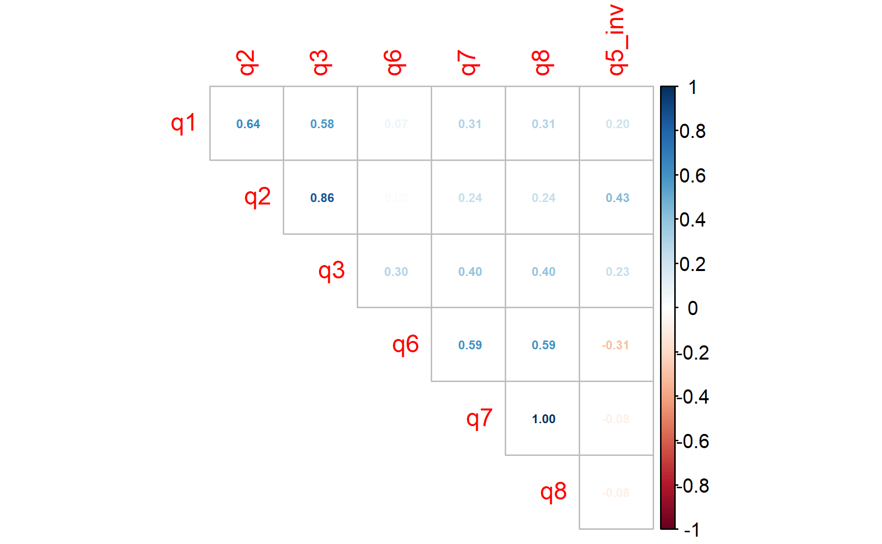
Items 1-3 are correlated as well as those evaluationg motivation (Q6-8). Item Q5, which was conflicting in prior analysis, here does not have any correlation.
As first approach the Barlett’s sphericity test is performed.
Thus, the p-value = 0 and the H0 is rejected confirming the utility of applying a factor analysis to this dataset.
Considering the fact that the Bartlett’s test usually rejects the H0 since the scenario of the null hypothesis is too extreme, the KMO analysis is studied to determine how well the data fit the factor analysis and how useful each item is.
## Error in solve.default(r) :
##   Lapack routine dgesv: system is exactly singular: U[7,7] = 0
## matrix is not invertible, image not found## Kaiser-Meyer-Olkin factor adequacy
## Call: KMO(r = pre_test_Q_Actitd_facAn_1_corr)
## Overall MSA = 0.5
## MSA for each item =
## q1 q2 q3 q4 q6 q7 q8 q5-inv
## 0.5 0.5 0.5 0.5 0.5 0.5 0.5 0.5The matrix is not invertible and the KMO cannot be calculated.
To explore the number of factors PCA and evaluate the variability explained for each component is considered. Thus, the table with the PCA results is shown below:
| PC1 | PC2 | PC3 | PC4 | PC5 | PC6 | PC7 | PC8 | |
|---|---|---|---|---|---|---|---|---|
| Standard deviation | 2.0138 | 1.4387 | 0.8599 | 0.6794 | 0.6181 | 0.4683 | 0.2691 | 0 |
| Proportion of Variance | 0.5069 | 0.2587 | 0.0924 | 0.0577 | 0.0478 | 0.0274 | 0.0091 | 0 |
| Cumulative Proportion | 0.5069 | 0.7657 | 0.8581 | 0.9158 | 0.9635 | 0.9910 | 1.0000 | 1 |
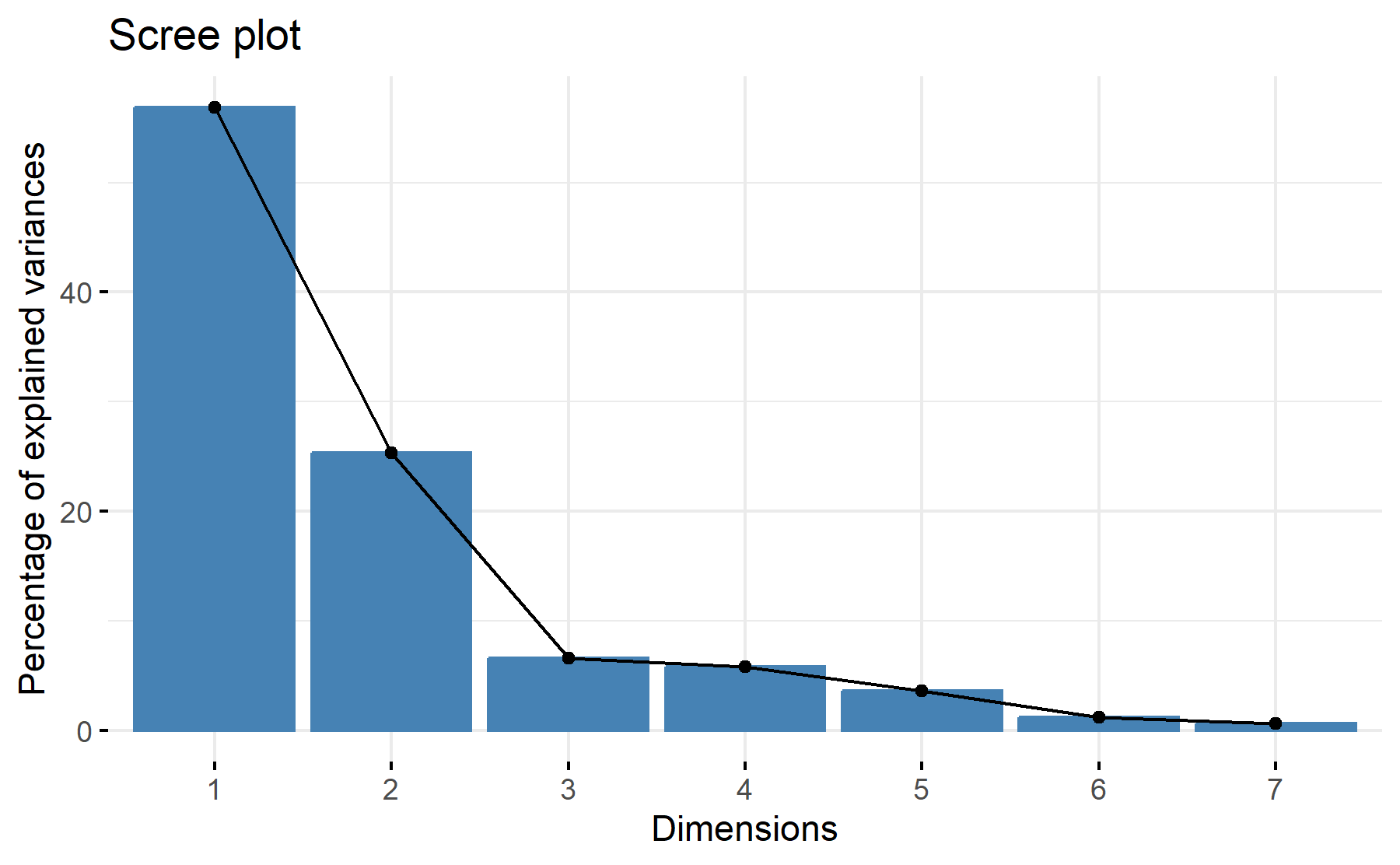
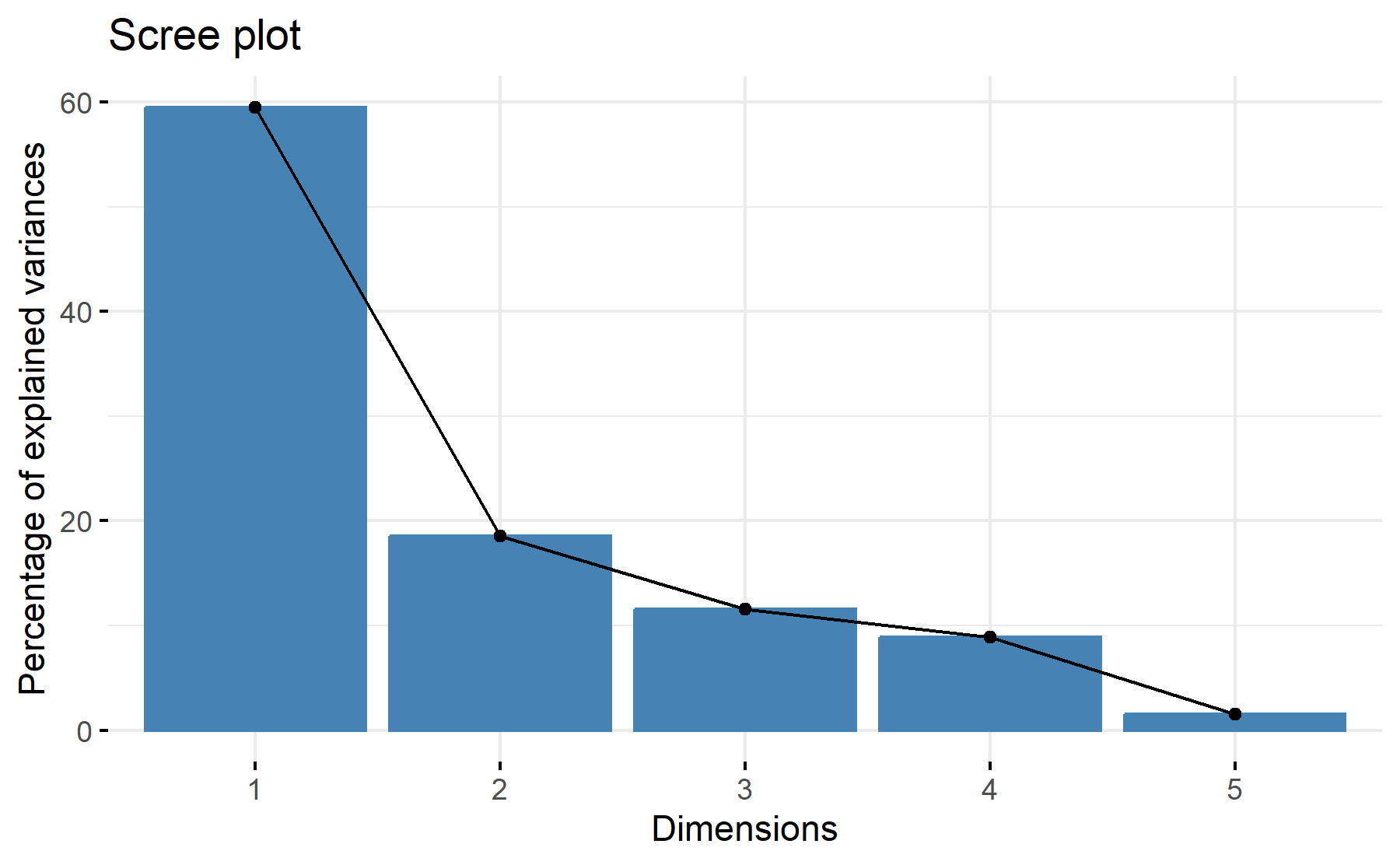
Then, the scree plot for this PCA analysis is displayed.
 According to these results, 2 or 3 factors could be adequate. With two 77% of the variability is explained.
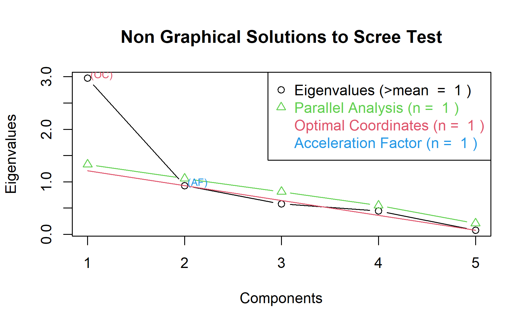
Then, another approach is implemented. With this strategy several analysis are combined and depict in the same figure. The tools implemented are: the Kaiser rule (which drops the components with eigenvalues < 1), the parallel analysis, and the usual scree test (plotuScree), the acceleration factor (which indicates where the elbow of the scree plot appears).
 Therefore, two factors will be considered.
Running the factor analysis with all the items (n=8), first the communalities are explored:
## Warning in cor.smooth(mat): Matrix was not positive definite, smoothing was
## done
## In factor.stats, I could not find the RMSEA upper bound . Sorry about that## In factor.scores, the correlation matrix is singular, the pseudo inverse is used## I was unable to calculate the factor score weights, factor loadings used instead## pre_actit_q1 pre_actit_q2 pre_actit_q3
## 0.5970 0.9950 0.9202
## pre_actit_q4 pre_actit_q6 pre_actit_q7
## 0.7857 0.9343 0.9950
## pre_actit_q8 pre_actit_q5_Inverted
## 0.9950 0.4544Therefore, considering the values of the communalities all the items are above 0.4.
Then, the whole output is displayed.
## Factor Analysis using method = ml
## Call: fa(r = pre_test_Q_Actitd_facAn_1, nfactors = 2, rotate = "oblimin",
## fm = "ml", cor = "poly")
## Standardized loadings (pattern matrix) based upon correlation matrix
## ML1 ML2 h2 u2 com
## pre_actit_q1 0.70 0.60 0.4032 1.1
## pre_actit_q2 1.01 1.00 0.0050 1.0
## pre_actit_q3 0.90 0.92 0.0799 1.1
## pre_actit_q4 0.67 0.42 0.79 0.2142 1.7
## pre_actit_q6 1.00 0.93 0.0657 1.0
## pre_actit_q7 0.98 1.00 0.0025 1.0
## pre_actit_q8 0.98 1.00 0.0025 1.0
## pre_actit_q5_Inverted -0.40 0.67 0.45 0.5466 1.6
##
## ML1 ML2
## SS loadings 3.65 3.03
## Proportion Var 0.46 0.38
## Cumulative Var 0.46 0.84
## Proportion Explained 0.55 0.45
## Cumulative Proportion 0.55 1.00
##
## With factor correlations of
## ML1 ML2
## ML1 1.0 0.3
## ML2 0.3 1.0
##
## Mean item complexity = 1.2
## Test of the hypothesis that 2 factors are sufficient.
##
## df null model = 28 with the objective function = 38.07 with Chi Square = 742.3
## df of the model are 13 and the objective function was 23.46
##
## The root mean square of the residuals (RMSR) is 0.05
## The df corrected root mean square of the residuals is 0.08
##
## The harmonic n.obs is 24 with the empirical chi square 3.56 with prob < 1
## The total n.obs was 24 with Likelihood Chi Square = 426.3 with prob < 0.000000000000000000000000000000000000000000000000000000000000000000000000000000000063
##
## Tucker Lewis Index of factoring reliability = -0.341
## RMSEA index = 1.15 and the 90 % confidence intervals are 1.081 NA
## BIC = 384.9
## Fit based upon off diagonal values = 0.99
## Measures of factor score adequacy
## ML1 ML2
## Correlation of (regression) scores with factors 1 1.00
## Multiple R square of scores with factors 1 1.00
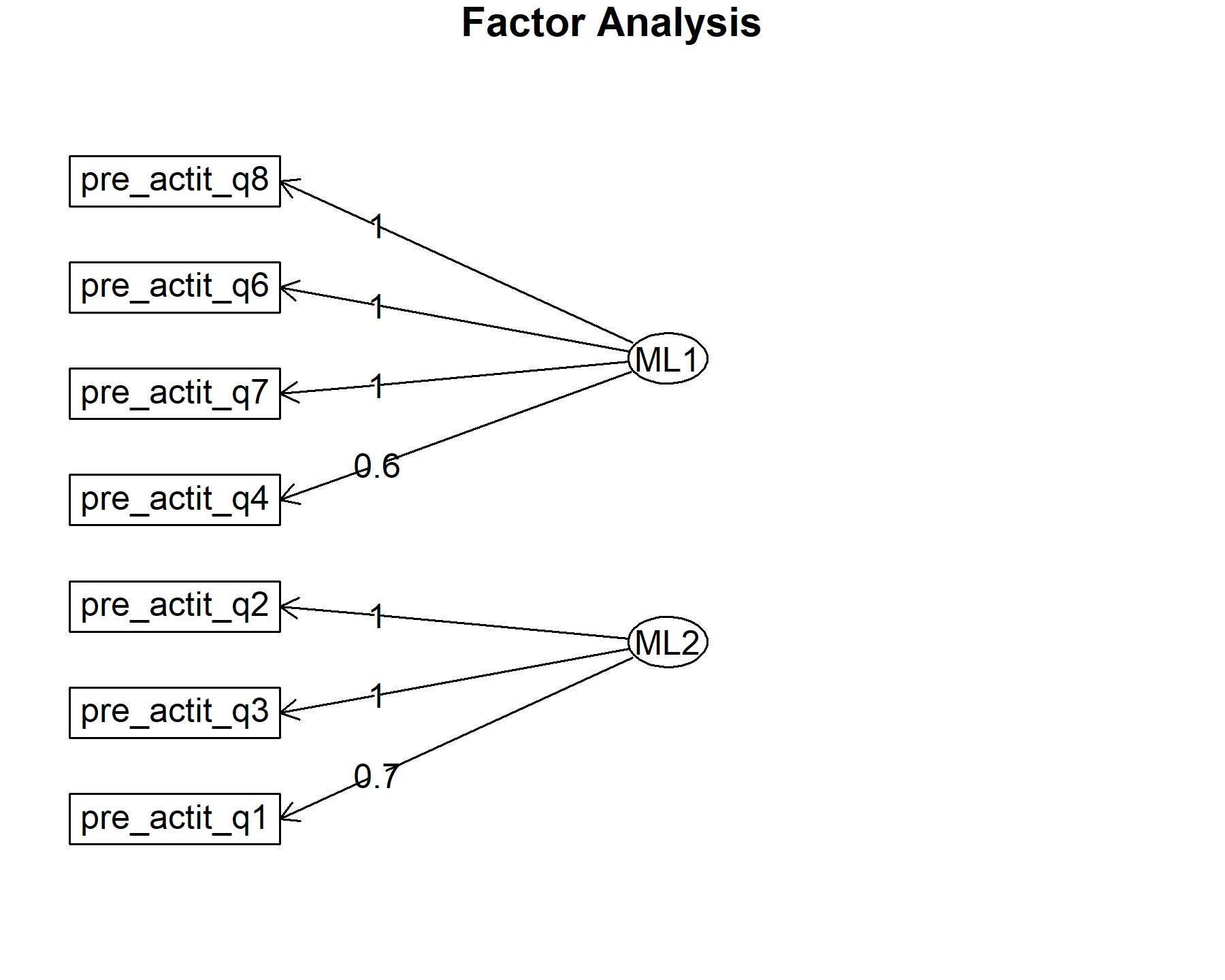
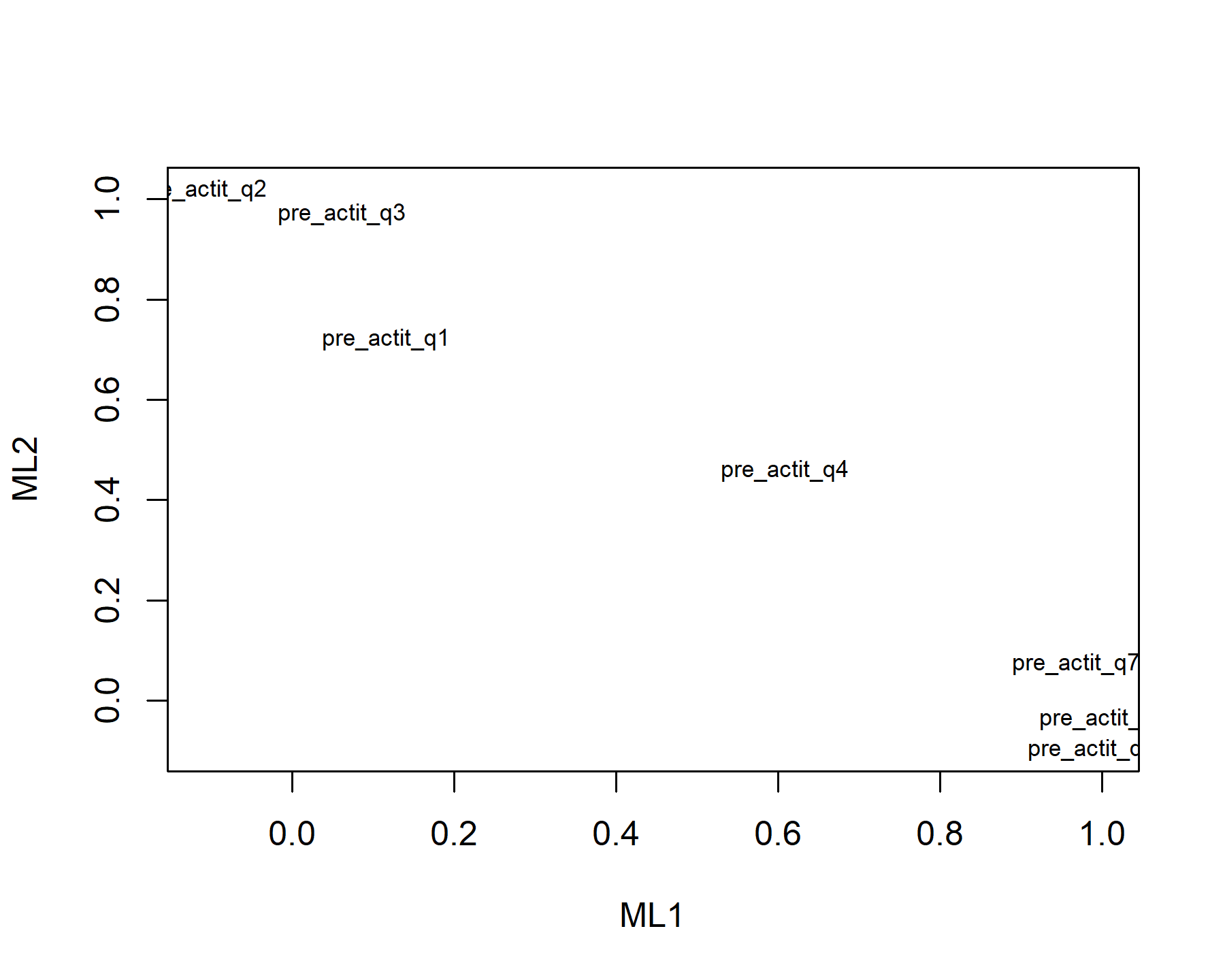
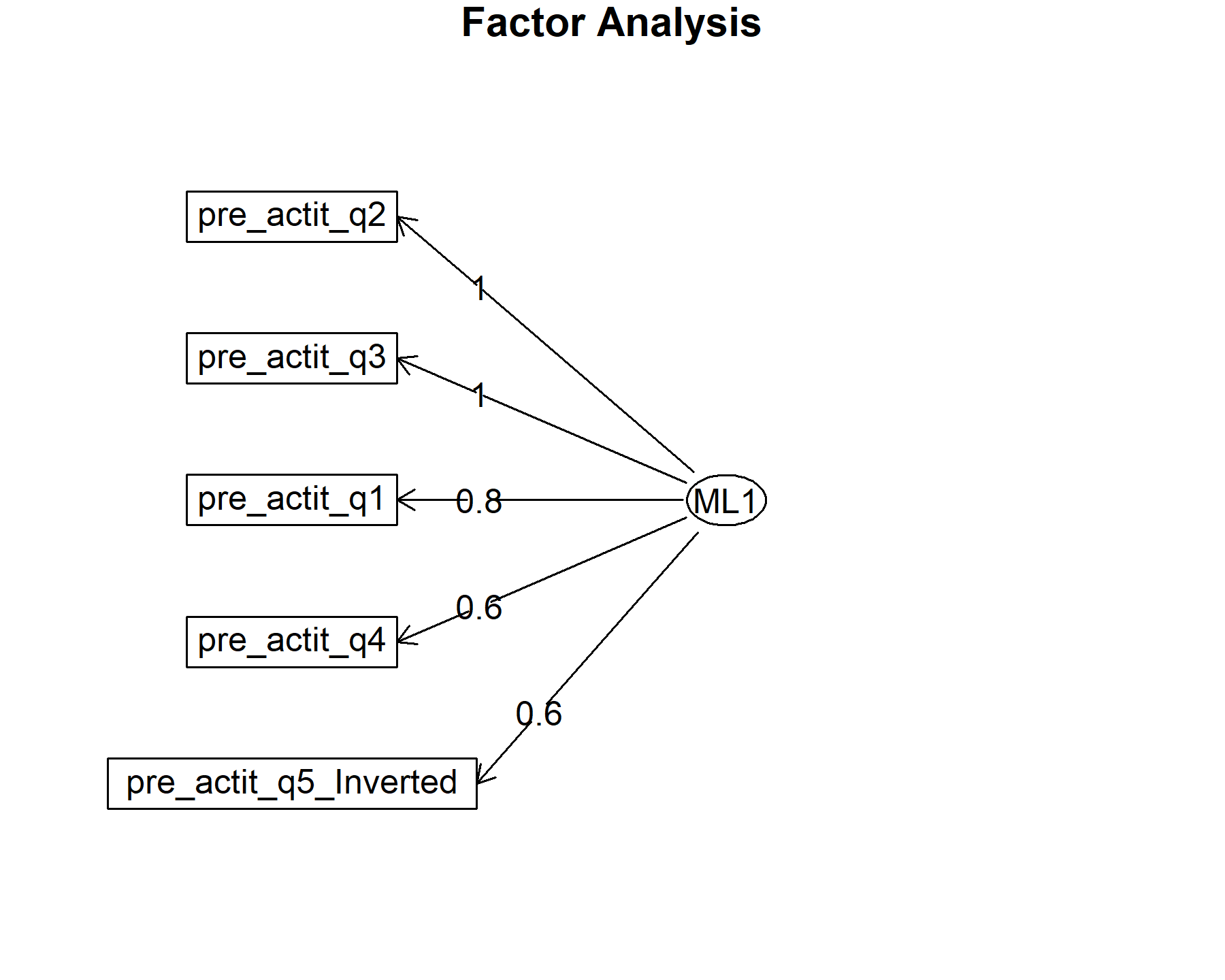
## Minimum correlation of possible factor scores 1 0.99Exploring these results, there are two factors composed by:
* Q6, Q7, and Q8.
* Q1, Q2, and Q3.
Both, Q4 and Q5 inv are presented in ML1 and 2.
Finally, plots show the relationship between the items and the factors.
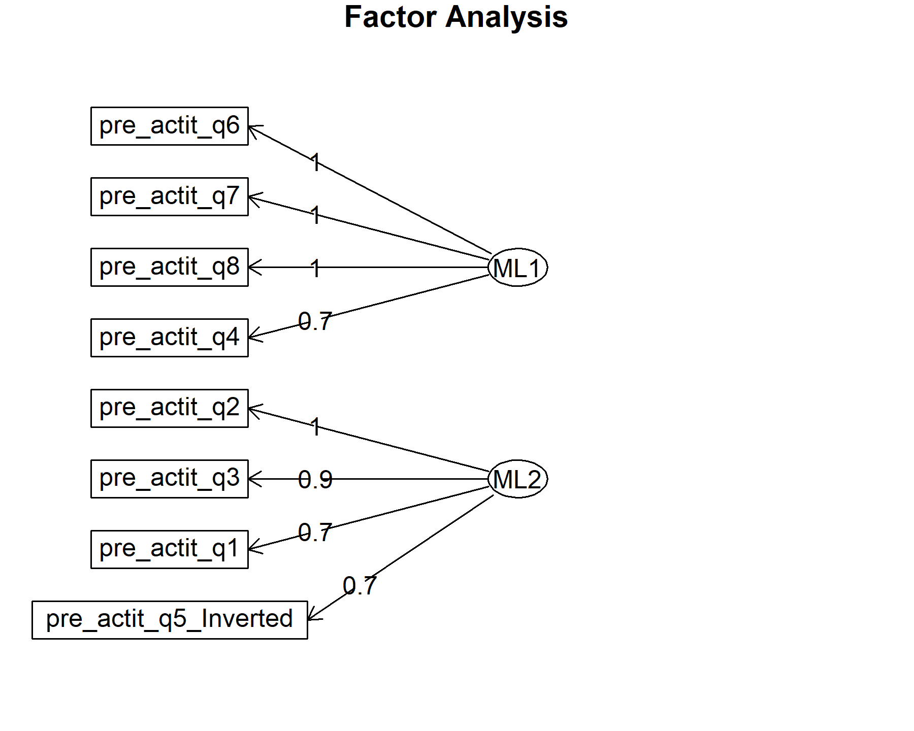
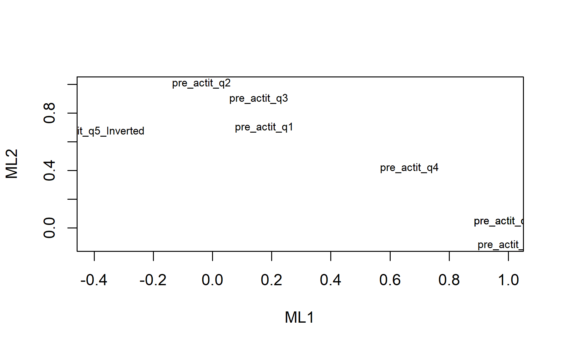
According to the factor analysis, two factors are found; one, is related to attitudes (Q1-3) and probably to the perception of benefit from genomic testing, and the other is related to motivation (Q6-8) and probably the perception of imprecision about the genomic testing (Q5 inv). In addition, when 3 factors were considered, instead of two, item 5 was identified as the unique element in this third factor. Taken all together, an approach could be choosing the first four items as the same domain, and the multiple option item as the other domain.
6.2.2 Excluding item 5.
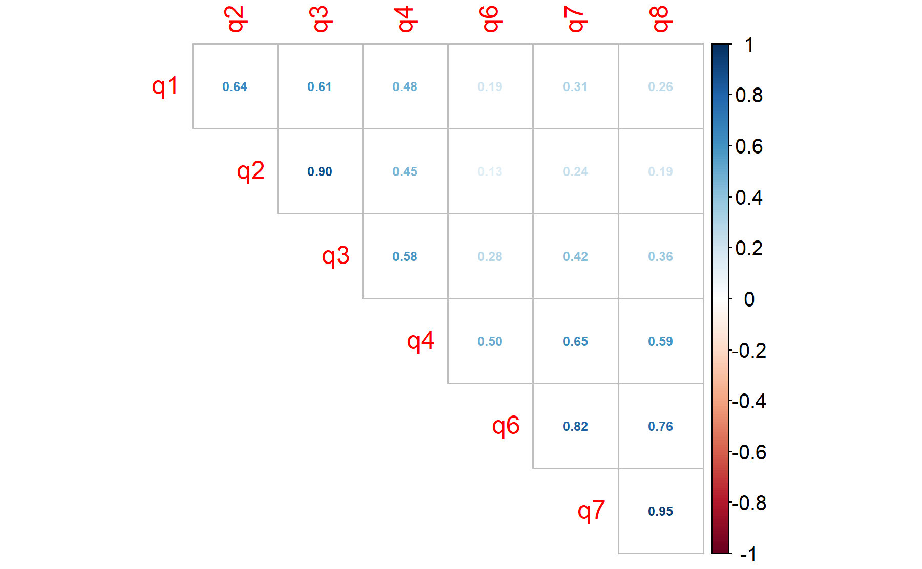
Items 1-3 are correlated as well as those evaluating motivation (Q6-8).
As first approach the Barlett’s sphericity test is performed.
Thus, the p-value = 0 and the H0 is rejected confirming the utility of applying a factor analysis to this dataset.
Considering the fact that the Bartlett’s test usually rejects the H0 since the scenario of the null hypothesis is too extreme, the KMO analysis is studied to determine how well the data fit the factor analysis and how useful each item is.
## Kaiser-Meyer-Olkin factor adequacy
## Call: KMO(r = pre_test_Q_Actitd_facAn_2_corr)
## Overall MSA =  0.76
## MSA for each item =
##   q1   q2   q3   q4   q6   q7   q8
## 0.90 0.65 0.71 0.94 0.88 0.70 0.74
All the values are above 0.7.
To explore the number of factors PCA and evaluate the variability explained for each component is considered. Thus, the table with the PCA results is shown below:
| PC1 | PC2 | PC3 | PC4 | PC5 | PC6 | PC7 | |
|---|---|---|---|---|---|---|---|
| Standard deviation | 1.9949 | 1.3312 | 0.6795 | 0.6383 | 0.5015 | 0.2888 | 0.2103 |
| Proportion of Variance | 0.5685 | 0.2532 | 0.0660 | 0.0582 | 0.0359 | 0.0119 | 0.0063 |
| Cumulative Proportion | 0.5685 | 0.8217 | 0.8876 | 0.9458 | 0.9818 | 0.9937 | 1.0000 |
Then, the scree plot for this PCA analysis is displayed.
 According to these results, 2 factors could be adequate. With two 77% of the variability is explained.
Then, another approach is implemented. With this strategy several analysis are combined and depict in the same figure. The tools implemented are: the Kaiser rule (which drops the components with eigenvalues < 1), the parallel analysis, and the usual scree test (plotuScree), the acceleration factor (which indicates where the elbow of the scree plot appears).
 Therefore, two factors will be considered.
Running the factor analysis with all the items (n=7), first the communalities are explored:
## Warning in cor.smooth(mat): Matrix was not positive definite, smoothing was
## done
## In factor.stats, I could not find the RMSEA upper bound . Sorry about that## pre_actit_q1 pre_actit_q2 pre_actit_q3 pre_actit_q4 pre_actit_q6 pre_actit_q7
## 0.5954 0.9689 0.9905 0.7851 0.9154 0.9950
## pre_actit_q8
## 0.9778Therefore, considering the values of the communalities all the items are above 0.4.
Then, the whole output is displayed.
## Factor Analysis using method =  ml
## Call: fa(r = pre_test_Q_Actitd_facAn_2, nfactors = 2, rotate = "oblimin",
##     fm = "ml", cor = "poly")
## Standardized loadings (pattern matrix) based upon correlation matrix
##                ML1   ML2   h2     u2 com
## pre_actit_q1        0.72 0.60 0.4046 1.1
## pre_actit_q2        1.02 0.97 0.0311 1.0
## pre_actit_q3        0.97 0.99 0.0095 1.0
## pre_actit_q4  0.61  0.46 0.79 0.2149 1.9
## pre_actit_q6  0.99       0.92 0.0846 1.0
## pre_actit_q7  0.97       1.00 0.0041 1.0
## pre_actit_q8  1.00       0.98 0.0222 1.0
##
##                        ML1  ML2
## SS loadings           3.41 2.82
## Proportion Var        0.49 0.40
## Cumulative Var        0.49 0.89
## Proportion Explained  0.55 0.45
## Cumulative Proportion 0.55 1.00
##
##  With factor correlations of
##      ML1  ML2
## ML1 1.00 0.36
## ML2 0.36 1.00
##
## Mean item complexity =  1.1
## Test of the hypothesis that 2 factors are sufficient.
##
## df null model =  21  with the objective function =  30.28 with Chi Square =  630.8
## df of  the model are 8  and the objective function was  18.21
##
## The root mean square of the residuals (RMSR) is  0.02
## The df corrected root mean square of the residuals is  0.03
##
## The harmonic n.obs is  25 with the empirical chi square  0.43  with prob <  1
## The total n.obs was  25  with Likelihood Chi Square =  355.1  with prob <  0.0000000000000000000000000000000000000000000000000000000000000000000000074
##
## Tucker Lewis Index of factoring reliability =  -0.6
## RMSEA index =  1.317  and the 90 % confidence intervals are  1.227 NA
## BIC =  329.3
## Fit based upon off diagonal values = 1
## Measures of factor score adequacy
##                                                    ML1  ML2
## Correlation of (regression) scores with factors   1.00 1.00
## Multiple R square of scores with factors          1.00 0.99
## Minimum correlation of possible factor scores     0.99 0.99
Exploring these results, there are three factors composed by:
* Q6, Q7, and Q8.
* Q1, Q2, and Q3.
Again, Q4 are presented in both.
Finally, plots show the relationship between the items and the factors.
 Now, although Q4 is related to both its loading is higher for ML1 and was located in the opposite factor comparing to the first analysis.
6.2.3 Excluding item 4 (preserving item 5 inverted).
Items 1-3 are correlated as well as those evaluating motivation (Q6-8).
As first approach the Barlett’s sphericity test is performed.
Thus, the p-value = 0 and the H0 is rejected confirming the utility of applying a factor analysis to this dataset.
Considering the fact that the Bartlett’s test usually rejects the H0 since the scenario of the null hypothesis is too extreme, the KMO analysis is studied to determine how well the data fit the factor analysis and how useful each item is.
## Error in solve.default(r) :
##   Lapack routine dgesv: system is exactly singular: U[6,6] = 0
## matrix is not invertible, image not found## Kaiser-Meyer-Olkin factor adequacy
## Call: KMO(r = pre_test_Q_Actitd_facAn_3_corr)
## Overall MSA = 0.5
## MSA for each item =
## q1 q2 q3 q6 q7 q8 q5_inv
## 0.5 0.5 0.5 0.5 0.5 0.5 0.5The matrix is not invertible and the KMO cannot be calculated.
To explore the number of factors PCA and evaluate the variability explained for each component is considered. Thus, the table with the PCA results is shown below:
| PC1 | PC2 | PC3 | PC4 | PC5 | PC6 | PC7 | |
|---|---|---|---|---|---|---|---|
| Standard deviation | 1.800 | 1.4187 | 0.8631 | 0.7443 | 0.5997 | 0.2955 | 0 |
| Proportion of Variance | 0.463 | 0.2875 | 0.1064 | 0.0791 | 0.0514 | 0.0125 | 0 |
| Cumulative Proportion | 0.463 | 0.7506 | 0.8570 | 0.9361 | 0.9875 | 1.0000 | 1 |
Then, the scree plot for this PCA analysis is displayed.
 According to these results, 2 factors could be adequate. With two 75% of the variability is explained.
Then, another approach is implemented. With this strategy several analysis are combined and depict in the same figure. The tools implemented are: the Kaiser rule (which drops the components with eigenvalues < 1), the parallel analysis, and the usual scree test (plotuScree), the acceleration factor (which indicates where the elbow of the scree plot appears).
 Therefore, two factors will be considered.
Running the factor analysis with all the items (n=7), first the communalities are explored:
## Warning in cor.smooth(mat): Matrix was not positive definite, smoothing was
## done
## In smc, smcs < 0 were set to .0
## In smc, smcs < 0 were set to .0## In factor.stats, I could not find the RMSEA upper bound . Sorry about that## In factor.scores, the correlation matrix is singular, the pseudo inverse is used## I was unable to calculate the factor score weights, factor loadings used instead## pre_actit_q1 pre_actit_q2 pre_actit_q3
## 0.6117 0.9950 0.8820
## pre_actit_q6 pre_actit_q7 pre_actit_q8
## 0.6996 0.9950 0.9950
## pre_actit_q5_Inverted
## 0.4516Therefore, considering the values of the communalities all the items are above 0.4, but Q5 showed the lower score (0.45).
Then, the whole output is displayed.
## Factor Analysis using method = ml
## Call: fa(r = pre_test_Q_Actitd_facAn_3, nfactors = 2, rotate = "oblimin",
## fm = "ml", cor = "poly")
## Standardized loadings (pattern matrix) based upon correlation matrix
## ML2 ML1 h2 u2 com
## pre_actit_q1 0.71 0.61 0.3884 1.1
## pre_actit_q2 1.00 1.00 0.0049 1.0
## pre_actit_q3 0.89 0.88 0.1180 1.1
## pre_actit_q6 0.86 0.70 0.3003 1.1
## pre_actit_q7 0.97 1.00 0.0025 1.0
## pre_actit_q8 0.97 1.00 0.0025 1.0
## pre_actit_q5_Inverted 0.67 0.45 0.5467 1.5
##
## ML2 ML1
## SS loadings 2.82 2.82
## Proportion Var 0.40 0.40
## Cumulative Var 0.40 0.81
## Proportion Explained 0.50 0.50
## Cumulative Proportion 0.50 1.00
##
## With factor correlations of
## ML2 ML1
## ML2 1.00 0.25
## ML1 0.25 1.00
##
## Mean item complexity = 1.1
## Test of the hypothesis that 2 factors are sufficient.
##
## df null model = 21 with the objective function = 34.92 with Chi Square = 727.6
## df of the model are 8 and the objective function was 23.69
##
## The root mean square of the residuals (RMSR) is 0.08
## The df corrected root mean square of the residuals is 0.13
##
## The harmonic n.obs is 25 with the empirical chi square 6.71 with prob < 0.57
## The total n.obs was 25 with Likelihood Chi Square = 462 with prob < 0.0000000000000000000000000000000000000000000000000000000000000000000000000000000000000000000001
##
## Tucker Lewis Index of factoring reliability = -0.805
## RMSEA index = 1.506 and the 90 % confidence intervals are 1.42 NA
## BIC = 436.2
## Fit based upon off diagonal values = 0.98
## Measures of factor score adequacy
## ML2 ML1
## Correlation of (regression) scores with factors 1.00 1.00
## Multiple R square of scores with factors 1.00 1.00
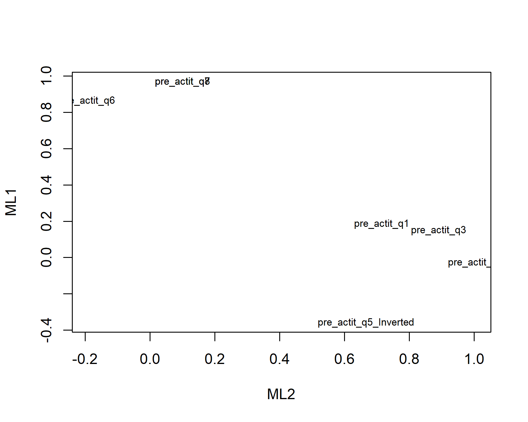
## Minimum correlation of possible factor scores 0.99 0.99Exploring these results, there are two factors composed by:
* Q1, Q2, and Q3, plus Q5 inv.
* Q6, Q7, and Q8.
Finally, plots show the relationship between the items and the factors.
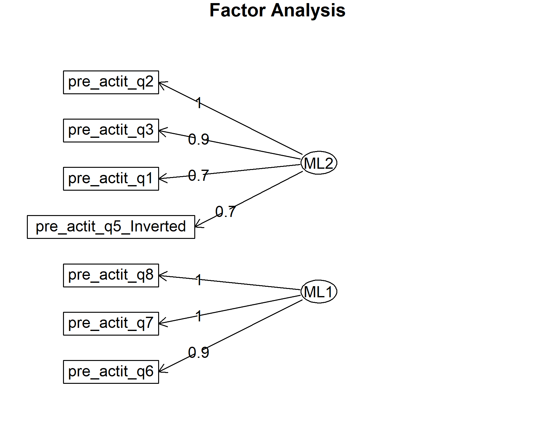
Again, attitudes items and motivation are located separately in different factors. Now, Q5 inv is related with the first factor with attitudes items.
6.2.4 Including Q1-Q5.
Now, motivation items are excluded.
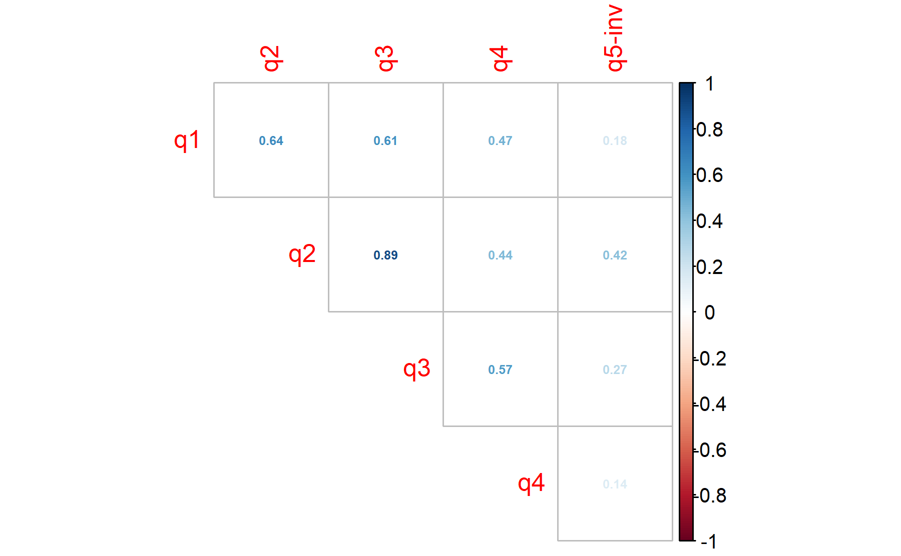
Item Q5 has only a moderate correlation with Q2 with no correlation with Q4.
As first approach the Barlett’s sphericity test is performed.
Thus, the p-value = 0 and the H0 is rejected confirming the utility of applying a factor analysis to this dataset.
Considering the fact that the Bartlett’s test usually rejects the H0 since the scenario of the null hypothesis is too extreme, the KMO analysis is studied to determine how well the data fit the factor analysis and how useful each item is.
## Kaiser-Meyer-Olkin factor adequacy
## Call: KMO(r = pre_test_Q_Actitd_facAn_4_corr)
## Overall MSA =  0.65
## MSA for each item =
##     q1     q2     q3     q4 q5-inv
##   0.84   0.60   0.62   0.71   0.53
All the items are above 0.5, only one is below 0.6.
To explore the number of factors PCA and evaluate the variability explained for each component is considered. Thus, the table with the PCA results is shown below:
| PC1 | PC2 | PC3 | PC4 | PC5 | |
|---|---|---|---|---|---|
| Standard deviation | 1.7243 | 0.9632 | 0.7603 | 0.6658 | 0.2788 |
| Proportion of Variance | 0.5946 | 0.1856 | 0.1156 | 0.0887 | 0.0156 |
| Cumulative Proportion | 0.5946 | 0.7802 | 0.8958 | 0.9844 | 1.0000 |
Then, the scree plot for this PCA analysis is displayed.
 According to these results, 1 or perhaps 2 factors could be adequate. With two 78% of the variability is explained.
Then, another approach is implemented. With this strategy several analysis are combined and depict in the same figure. The tools implemented are: the Kaiser rule (which drops the components with eigenvalues < 1), the parallel analysis, and the usual scree test (plotuScree), the acceleration factor (which indicates where the elbow of the scree plot appears).
 Therefore, one factor will be considered.
Running the factor analysis with all the items (n=5), first the communalities are explored:
## Warning in cor.smooth(mat): Matrix was not positive definite, smoothing was
## done
## In smc, smcs < 0 were set to .0
## In smc, smcs < 0 were set to .0## In factor.stats, I could not find the RMSEA upper bound . Sorry about that## pre_actit_q1 pre_actit_q2 pre_actit_q3
## 0.5660 0.9950 0.9077
## pre_actit_q4 pre_actit_q5_Inverted
## 0.3594 0.3195Therefore, considering the values of the communalities all the items are above 0.3.
Then, the whole output is displayed.
## Factor Analysis using method =  ml
## Call: fa(r = pre_test_Q_Actitd_facAn_4, nfactors = 1, rotate = "oblimin",
##     fm = "ml", cor = "poly")
## Standardized loadings (pattern matrix) based upon correlation matrix
##                        ML1   h2    u2 com
## pre_actit_q1          0.75 0.57 0.434   1
## pre_actit_q2          1.00 1.00 0.005   1
## pre_actit_q3          0.95 0.91 0.092   1
## pre_actit_q4          0.60 0.36 0.641   1
## pre_actit_q5_Inverted 0.57 0.32 0.680   1
##
##                 ML1
## SS loadings    3.15
## Proportion Var 0.63
##
## Mean item complexity =  1
## Test of the hypothesis that 1 factor is sufficient.
##
## df null model =  10  with the objective function =  24.03 with Chi Square =  492.6
## df of  the model are 5  and the objective function was  20.04
##
## The root mean square of the residuals (RMSR) is  0.11
## The df corrected root mean square of the residuals is  0.15
##
## The harmonic n.obs is  24 with the empirical chi square  5.54  with prob <  0.35
## The total n.obs was  24  with Likelihood Chi Square =  397.4  with prob <  0.000000000000000000000000000000000000000000000000000000000000000000000000000000000011
##
## Tucker Lewis Index of factoring reliability =  -0.682
## RMSEA index =  1.808  and the 90 % confidence intervals are  1.696 NA
## BIC =  381.6
## Fit based upon off diagonal values = 0.97
## Measures of factor score adequacy
##                                                    ML1
## Correlation of (regression) scores with factors   1.00
## Multiple R square of scores with factors          1.00
## Minimum correlation of possible factor scores     0.99
Exploring these results, there is one factor composed by:
* Composed by all the items (Q1-Q5).
The lowest loading is for Q5 with 0.57 followed by Q4 with 0.60. The total variance explained is 0.63.
Finally, plots show the relationship between the items and the factors.
6.2.5 Conclusion
Three options could be considered:
1. Items Q1-3 + Q4 and Q5 + item 9 with multiple options.
2. Items Q1-3 + Q5 + item 9 with multiple options.
3. Items Q1-3 + Q4 + item 9 with multiple options.
The positive effect of the 2nd approach is having a inverted item, but this Q5 showed some issues during the first analysis. On the other hand, the third strategy could be better but perhaps less informative.
6.3 Both domains, the expectations and concerns domain plus the attitudes domain
6.3.1 Expectations plus Q2 and Q3 from attitudes.
Including all the items selected for expectations (Q2, Q5, Q6, Q7.i, Q7.iv, Q7.v, Q8, Q9, 10, and Q11), plus two items from the attitude domain (Q2 and Q3).
The Barlett’s sphericity test is performed.
Thus, the p-value = 0 and the H0 is rejected confirming the utility of applying a factor analysis to this dataset.
Considering the fact that the Bartlett’s test usually rejects the H0 since the scenario of the null hypothesis is too extreme, the KMO analysis is studied to determine how well the data fit the factor analysis and how useful each item is.
## Kaiser-Meyer-Olkin factor adequacy
## Call: KMO(r = pre_test_Q_Exp_Attit_facAn_1_corr)
## Overall MSA =  0.64
## MSA for each item =
##       q2       q5       q6     q7_i    q7_iv     q7_v       q8       q9
##     0.70     0.60     0.63     0.69     0.66     0.66     0.68     0.62
##      q10      q11 actit_q2 actit_q3
##     0.56     0.73     0.56     0.67
According to these results, there is no items under the threshold of 0.5. Two items are below 0.6.
To explore the number of factors PCA is applied. Thus, the table with the PCA results is shown below:
| PC1 | PC2 | PC3 | PC4 | PC5 | PC6 | PC7 | PC8 | PC9 | PC10 | PC11 | PC12 | |
|---|---|---|---|---|---|---|---|---|---|---|---|---|
| Standard deviation | 2.023 | 1.9119 | 1.2291 | 0.7759 | 0.7453 | 0.6567 | 0.6098 | 0.5580 | 0.4418 | 0.3863 | 0.2685 | 0.2304 |
| Proportion of Variance | 0.341 | 0.3046 | 0.1259 | 0.0502 | 0.0463 | 0.0359 | 0.0310 | 0.0260 | 0.0163 | 0.0124 | 0.0060 | 0.0044 |
| Cumulative Proportion | 0.341 | 0.6456 | 0.7715 | 0.8217 | 0.8680 | 0.9039 | 0.9349 | 0.9609 | 0.9771 | 0.9896 | 0.9956 | 1.0000 |
Then, the scree plot for this PCA analysis is displayed.
 According to these results, 3 factors could be the best number. The cumulative proportion showed that with 3 components 77%, there are two elbows, one after two and the other on the third component.
Then, another approach is implemented. With this strategy several analysis are combined and depict in the same figure. The tools implemented are: the Kaiser rule (which drops the components with eigenvalues < 1), the parallel analysis, and the usual scree test (plotuScree), the acceleration factor (which indicates where the elbow of the scree plot appears).
 Therefore, considering three factors seem to be an adequate approach.
Running the factor analysis with 12 items, first the communalities are explored:
## Warning in cor.smooth(mat): Matrix was not positive definite, smoothing was
## done
## In factor.stats, I could not find the RMSEA upper bound . Sorry about that## pre_exp_preoc_q2 pre_exp_preoc_q5 pre_exp_preoc_q6 pre_exp_preoc_q7_i
## 0.7043 0.8482 0.9534 0.7732
## pre_exp_preoc_q7_iv pre_exp_preoc_q7_v pre_exp_preoc_q8 pre_exp_preoc_q9
## 0.9950 0.7092 0.7629 0.6177
## pre_exp_preoc_q10 pre_exp_preoc_q11 pre_actit_q2 pre_actit_q3
## 0.6972 0.7771 0.9371 0.9629Considering the values of the communalities, all are above 0.3.
Then, the whole output is displayed.
## Factor Analysis using method =  ml
## Call: fa(r = pre_test_Q_Exp_Attit_facAn_1, nfactors = 3, rotate = "oblimin",
##     fm = "ml", cor = "poly")
## Standardized loadings (pattern matrix) based upon correlation matrix
##                       ML2   ML3   ML1   h2     u2 com
## pre_exp_preoc_q2     0.70             0.70 0.2956 1.4
## pre_exp_preoc_q5                 0.85 0.85 0.1518 1.2
## pre_exp_preoc_q6                 1.02 0.95 0.0466 1.0
## pre_exp_preoc_q7_i   0.87             0.77 0.2266 1.2
## pre_exp_preoc_q7_iv              0.84 1.00 0.0048 1.4
## pre_exp_preoc_q7_v   0.63             0.71 0.2911 2.1
## pre_exp_preoc_q8           0.90       0.76 0.2370 1.0
## pre_exp_preoc_q9           0.73       0.62 0.3825 1.1
## pre_exp_preoc_q10          0.79       0.70 0.3030 1.2
## pre_exp_preoc_q11          0.84       0.78 0.2229 1.0
## pre_actit_q2         0.95             0.94 0.0629 1.1
## pre_actit_q3         0.94             0.96 0.0371 1.0
##
##                        ML2  ML3  ML1
## SS loadings           3.67 3.22 2.85
## Proportion Var        0.31 0.27 0.24
## Cumulative Var        0.31 0.57 0.81
## Proportion Explained  0.38 0.33 0.29
## Cumulative Proportion 0.38 0.71 1.00
##
##  With factor correlations of
##       ML2   ML3  ML1
## ML2  1.00 -0.16 0.33
## ML3 -0.16  1.00 0.25
## ML1  0.33  0.25 1.00
##
## Mean item complexity =  1.2
## Test of the hypothesis that 3 factors are sufficient.
##
## df null model =  66  with the objective function =  74.6 with Chi Square =  1430
## df of  the model are 33  and the objective function was  60.9
##
## The root mean square of the residuals (RMSR) is  0.05
## The df corrected root mean square of the residuals is  0.07
##
## The harmonic n.obs is  25 with the empirical chi square  7.44  with prob <  1
## The total n.obs was  25  with Likelihood Chi Square =  1045  with prob <  2.7e-198
##
## Tucker Lewis Index of factoring reliability =  -0.667
## RMSEA index =  1.107  and the 90 % confidence intervals are  1.072 NA
## BIC =  939.2
## Fit based upon off diagonal values = 0.99
## Measures of factor score adequacy
##                                                    ML2  ML3  ML1
## Correlation of (regression) scores with factors   0.99 0.97 0.99
## Multiple R square of scores with factors          0.98 0.95 0.99
## Minimum correlation of possible factor scores     0.96 0.90 0.98
There are 3 factors:
* Q2, Q7_i, Q7_v, attQ2, attQ3.
* Q5, Q6, Q7_iv.
* Q8, Q9, Q10, Q11.
Finally, plots show the relationship between the items and the factors.

6.3.2 Expectations plus Q2, Q3, Q4, and Q5 inv from attitudes.
Including all the items selected for expectations (Q2, Q5, Q6, Q7.i, Q7.iv, Q7.v, Q8, Q9, 10, and Q11), plus four items from the attitude domain (Q2, Q3, Q4, and Q5 inverted).
The Barlett’s sphericity test is performed.
Thus, the p-value = 0 and the H0 is rejected confirming the utility of applying a factor analysis to this dataset.
Considering the fact that the Bartlett’s test usually rejects the H0 since the scenario of the null hypothesis is too extreme, the KMO analysis is studied to determine how well the data fit the factor analysis and how useful each item is.
## Kaiser-Meyer-Olkin factor adequacy
## Call: KMO(r = pre_test_Q_Exp_Attit_facAn_2_corr)
## Overall MSA =  0.61
## MSA for each item =
##           q2           q5           q6         q7_i        q7_iv         q7_v
##         0.76         0.67         0.55         0.57         0.67         0.46
##           q8           q9          q10          q11     actit_q2     actit_q3
##         0.52         0.58         0.51         0.80         0.65         0.67
##     actit_q4 actit_q5_Inv
##         0.73         0.53
According to these results, there is one item under the threshold of 0.5 (q7_v). Six items are below 0.6.
To explore the number of factors PCA is applied. Thus, the table with the PCA results is shown below:
| PC1 | PC2 | PC3 | PC4 | PC5 | PC6 | PC7 | PC8 | PC9 | PC10 | PC11 | PC12 | PC13 | PC14 | |
|---|---|---|---|---|---|---|---|---|---|---|---|---|---|---|
| Standard deviation | 2.2233 | 1.8626 | 1.3819 | 0.8605 | 0.8470 | 0.7602 | 0.6753 | 0.5996 | 0.5481 | 0.4938 | 0.3672 | 0.2475 | 0.2267 | 0.1869 |
| Proportion of Variance | 0.3531 | 0.2478 | 0.1364 | 0.0529 | 0.0512 | 0.0413 | 0.0326 | 0.0257 | 0.0215 | 0.0174 | 0.0096 | 0.0044 | 0.0037 | 0.0025 |
| Cumulative Proportion | 0.3531 | 0.6009 | 0.7373 | 0.7902 | 0.8414 | 0.8827 | 0.9153 | 0.9410 | 0.9624 | 0.9798 | 0.9895 | 0.9938 | 0.9975 | 1.0000 |
Then, the scree plot for this PCA analysis is displayed.
 According to these results, 3-4 factors could be the best number. The cumulative proportion showed that with 3 components 74% and 79% with four. The greatest elbow is on the four component.
Then, another approach is implemented. With this strategy several analysis are combined and depict in the same figure. The tools implemented are: the Kaiser rule (which drops the components with eigenvalues < 1), the parallel analysis, and the usual scree test (plotuScree), the acceleration factor (which indicates where the elbow of the scree plot appears).
 Therefore, considering three factors seem to be an adequate approach.
Running the factor analysis with 14 items, first the communalities are explored:
## Warning in cor.smooth(mat): Matrix was not positive definite, smoothing was
## done
## In smc, smcs < 0 were set to .0
## In smc, smcs < 0 were set to .0## In factor.stats, I could not find the RMSEA upper bound . Sorry about that## pre_exp_preoc_q2 pre_exp_preoc_q5 pre_exp_preoc_q6
## 0.8616 0.8974 0.9731
## pre_exp_preoc_q7_i pre_exp_preoc_q7_iv pre_exp_preoc_q7_v
## 0.9950 0.9950 0.6193
## pre_exp_preoc_q8 pre_exp_preoc_q9 pre_exp_preoc_q10
## 0.6864 0.5281 0.7194
## pre_exp_preoc_q11 pre_actit_q2 pre_actit_q3
## 0.7535 0.8810 0.8167
## pre_actit_q4 pre_actit_q5_Inverted
## 0.6180 0.6246Considering the values of the communalities, all are above 0.3.
Then, the whole output is displayed.
## Factor Analysis using method =  ml
## Call: fa(r = pre_test_Q_Exp_Attit_facAn_2, nfactors = 3, rotate = "oblimin",
##     fm = "ml", cor = "poly")
## Standardized loadings (pattern matrix) based upon correlation matrix
##                         ML2   ML3   ML1   h2     u2 com
## pre_exp_preoc_q2       0.77             0.86 0.1384 1.4
## pre_exp_preoc_q5                   0.86 0.90 0.1024 1.3
## pre_exp_preoc_q6                   1.00 0.97 0.0269 1.0
## pre_exp_preoc_q7_i     1.06             1.00 0.0049 1.1
## pre_exp_preoc_q7_iv          0.50  0.83 1.00 0.0049 1.6
## pre_exp_preoc_q7_v     0.65             0.62 0.3804 1.8
## pre_exp_preoc_q8             0.85       0.69 0.3142 1.1
## pre_exp_preoc_q9             0.70       0.53 0.4661 1.1
## pre_exp_preoc_q10            0.79       0.72 0.2813 1.1
## pre_exp_preoc_q11            0.85       0.75 0.2460 1.0
## pre_actit_q2           0.85             0.88 0.1188 1.2
## pre_actit_q3           0.81             0.82 0.1841 1.1
## pre_actit_q4           0.67             0.62 0.3803 1.3
## pre_actit_q5_Inverted       -0.63       0.62 0.3752 1.6
##
##                        ML2  ML3  ML1
## SS loadings           4.43 3.64 2.90
## Proportion Var        0.32 0.26 0.21
## Cumulative Var        0.32 0.58 0.78
## Proportion Explained  0.40 0.33 0.26
## Cumulative Proportion 0.40 0.74 1.00
##
##  With factor correlations of
##       ML2   ML3  ML1
## ML2  1.00 -0.22 0.27
## ML3 -0.22  1.00 0.07
## ML1  0.27  0.07 1.00
##
## Mean item complexity =  1.3
## Test of the hypothesis that 3 factors are sufficient.
##
## df null model =  91  with the objective function =  97.53 with Chi Square =  1609
## df of  the model are 52  and the objective function was  81.71
##
## The root mean square of the residuals (RMSR) is  0.06
## The df corrected root mean square of the residuals is  0.08
##
## The harmonic n.obs is  23 with the empirical chi square  14.47  with prob <  1
## The total n.obs was  23  with Likelihood Chi Square =  1185  with prob <  7.4e-214
##
## Tucker Lewis Index of factoring reliability =  -0.498
## RMSEA index =  0.972  and the 90 % confidence intervals are  0.946 NA
## BIC =  1022
## Fit based upon off diagonal values = 0.98
## Measures of factor score adequacy
##                                                    ML2  ML3  ML1
## Correlation of (regression) scores with factors   1.00 0.98 0.99
## Multiple R square of scores with factors          0.99 0.97 0.99
## Minimum correlation of possible factor scores     0.99 0.94 0.98
There are 3 factors:
* Q2, Q7_i, Q7_v, attQ2, attQ3, attQ4.
* Q5, Q6, Q7_iv.
* Q8, Q9, Q10, Q11, Q7_iv, attQ5 inv.
Even when items from attitudes are mixed with expectations, there is a conceptual relationship between them. Besides, the negative loading of Q5 makes sense with concerns.
Finally, plots show the relationship between the items and the factors.
6.3.3 Expectations plus Q2, Q3, and Q4 from attitudes.
Including all the items selected for expectations (Q2, Q5, Q6, Q7.i, Q7.iv, Q7.v, Q8, Q9, 10, and Q11), plus three items from the attitude domain (Q2, Q3, and Q4).
The Barlett’s sphericity test is performed.
Thus, the p-value = 0 and the H0 is rejected confirming the utility of applying a factor analysis to this dataset.
Considering the fact that the Bartlett’s test usually rejects the H0 since the scenario of the null hypothesis is too extreme, the KMO analysis is studied to determine how well the data fit the factor analysis and how useful each item is.
## Kaiser-Meyer-Olkin factor adequacy
## Call: KMO(r = pre_test_Q_Exp_Attit_facAn_3_corr)
## Overall MSA =  0.69
## MSA for each item =
##       q2       q5       q6     q7_i    q7_iv     q7_v       q8       q9
##     0.75     0.66     0.61     0.77     0.61     0.68     0.71     0.62
##      q10      q11 actit_q2 actit_q3 actit_q4
##     0.59     0.71     0.68     0.71     0.79
According to these results, there is no items under the threshold of 0.5. One item is below 0.6.
To explore the number of factors PCA is applied. Thus, the table with the PCA results is shown below:
| PC1 | PC2 | PC3 | PC4 | PC5 | PC6 | PC7 | PC8 | PC9 | PC10 | PC11 | PC12 | PC13 | |
|---|---|---|---|---|---|---|---|---|---|---|---|---|---|
| Standard deviation | 2.1555 | 1.8185 | 1.3641 | 0.8423 | 0.7515 | 0.7050 | 0.6256 | 0.5872 | 0.5008 | 0.4077 | 0.3638 | 0.2792 | 0.2262 |
| Proportion of Variance | 0.3574 | 0.2544 | 0.1431 | 0.0546 | 0.0435 | 0.0382 | 0.0301 | 0.0265 | 0.0193 | 0.0128 | 0.0102 | 0.0060 | 0.0039 |
| Cumulative Proportion | 0.3574 | 0.6118 | 0.7549 | 0.8095 | 0.8529 | 0.8912 | 0.9213 | 0.9478 | 0.9671 | 0.9799 | 0.9901 | 0.9961 | 1.0000 |
Then, the scree plot for this PCA analysis is displayed.
 According to these results, 3-4 factors could be the best number. The cumulative proportion showed that with 3 components 75% and 81% with four. The greatest elbow is on the four component.
Then, another approach is implemented. With this strategy several analysis are combined and depict in the same figure. The tools implemented are: the Kaiser rule (which drops the components with eigenvalues < 1), the parallel analysis, and the usual scree test (plotuScree), the acceleration factor (which indicates where the elbow of the scree plot appears).
 Therefore, considering three factors seem to be an adequate approach.
Running the factor analysis with 13 items, first the communalities are explored:
## Warning in cor.smooth(mat): Matrix was not positive definite, smoothing was
## done
## In factor.stats, I could not find the RMSEA upper bound . Sorry about that## pre_exp_preoc_q2 pre_exp_preoc_q5 pre_exp_preoc_q6 pre_exp_preoc_q7_i
## 0.8800 0.9316 0.9271 0.9950
## pre_exp_preoc_q7_iv pre_exp_preoc_q7_v pre_exp_preoc_q8 pre_exp_preoc_q9
## 0.9817 0.6500 0.7389 0.5678
## pre_exp_preoc_q10 pre_exp_preoc_q11 pre_actit_q2 pre_actit_q3
## 0.7577 0.7799 0.8639 0.8234
## pre_actit_q4
## 0.6682Considering the values of the communalities, all are above 0.3.
Then, the whole output is displayed.
## Factor Analysis using method =  ml
## Call: fa(r = pre_test_Q_Exp_Attit_facAn_3, nfactors = 3, rotate = "oblimin",
##     fm = "ml", cor = "poly")
## Standardized loadings (pattern matrix) based upon correlation matrix
##                       ML1   ML3   ML2   h2     u2 com
## pre_exp_preoc_q2     0.79             0.88 0.1201 1.3
## pre_exp_preoc_q5                 0.85 0.93 0.0684 1.3
## pre_exp_preoc_q6                 0.98 0.93 0.0729 1.0
## pre_exp_preoc_q7_i   1.06             1.00 0.0049 1.1
## pre_exp_preoc_q7_iv        0.48  0.82 0.98 0.0183 1.6
## pre_exp_preoc_q7_v   0.67             0.65 0.3490 1.8
## pre_exp_preoc_q8           0.88       0.74 0.2610 1.1
## pre_exp_preoc_q9           0.73       0.57 0.4327 1.1
## pre_exp_preoc_q10          0.79       0.76 0.2421 1.2
## pre_exp_preoc_q11          0.86       0.78 0.2204 1.1
## pre_actit_q2         0.88             0.86 0.1361 1.1
## pre_actit_q3         0.83             0.82 0.1766 1.1
## pre_actit_q4         0.68             0.67 0.3316 1.3
##
##                        ML1  ML3  ML2
## SS loadings           4.43 3.27 2.86
## Proportion Var        0.34 0.25 0.22
## Cumulative Var        0.34 0.59 0.81
## Proportion Explained  0.42 0.31 0.27
## Cumulative Proportion 0.42 0.73 1.00
##
##  With factor correlations of
##       ML1   ML3  ML2
## ML1  1.00 -0.18 0.27
## ML3 -0.18  1.00 0.08
## ML2  0.27  0.08 1.00
##
## Mean item complexity =  1.2
## Test of the hypothesis that 3 factors are sufficient.
##
## df null model =  78  with the objective function =  77.04 with Chi Square =  1374
## df of  the model are 42  and the objective function was  62
##
## The root mean square of the residuals (RMSR) is  0.05
## The df corrected root mean square of the residuals is  0.07
##
## The harmonic n.obs is  24 with the empirical chi square  8.91  with prob <  1
## The total n.obs was  24  with Likelihood Chi Square =  981.7  with prob <  1.9e-178
##
## Tucker Lewis Index of factoring reliability =  -0.528
## RMSEA index =  0.965  and the 90 % confidence intervals are  0.933 NA
## BIC =  848.2
## Fit based upon off diagonal values = 0.99
## Measures of factor score adequacy
##                                                    ML1  ML3  ML2
## Correlation of (regression) scores with factors   1.00 0.98 0.99
## Multiple R square of scores with factors          0.99 0.96 0.98
## Minimum correlation of possible factor scores     0.99 0.91 0.97
There are 3 factors:
* Q2, Q7_i, Q7_v, attQ2, attQ3, attQ4.
* Q5, Q6, Q7_iv.
* Q8, Q9, Q10, Q11, Q7_iv.
No additional effect is detected when item 5 is excluded.
Finally, plots show the relationship between the items and the factors.
6.3.4 Evaluating the presence of outliers
As an exploratory approach, the possibility of being a patient that answered all the items with “totally agree” is analyzed. Considering the small number of patients, and some behavior of the items along with the lack of complementary with the HOPE study with possibility is considered.
First, the existence of cases with this pattern is checked.
There is a patient (ID 27) who answer all the items with 5 (Totalmente de acuerdo)
6.3.4.1 Expectations plus Q2 and Q3 from attitudes.
The factor analysis is run again with the best combination of items. Including all the items selected for expectations plus Q2 and Q3 from attitudes.

The Barlett’s sphericity test is performed.
Thus, the p-value = 0 and the H0 is rejected confirming the utility of applying a factor analysis to this dataset.
Considering the fact that the Bartlett’s test usually rejects the H0 since the scenario of the null hypothesis is too extreme, the KMO analysis is studied to determine how well the data fit the factor analysis and how useful each item is.
## Kaiser-Meyer-Olkin factor adequacy
## Call: KMO(r = pre_test_Q_Exp_Attit_facAn_4_corr)
## Overall MSA =  0.65
## MSA for each item =
##       q2       q5       q6     q7_i    q7_iv     q7_v       q8       q9
##     0.71     0.60     0.62     0.70     0.67     0.64     0.67     0.60
##      q10      q11 actit_q2 actit_q3
##     0.59     0.73     0.58     0.69
According to these results, there is no items under the threshold of 0.5. Two items are below 0.6.
To explore the number of factors PCA is applied. Thus, the table with the PCA results is shown below:
| PC1 | PC2 | PC3 | PC4 | PC5 | PC6 | PC7 | PC8 | PC9 | PC10 | PC11 | PC12 | |
|---|---|---|---|---|---|---|---|---|---|---|---|---|
| Standard deviation | 2.0216 | 1.8952 | 1.2310 | 0.7743 | 0.7618 | 0.6745 | 0.6202 | 0.5649 | 0.4302 | 0.3908 | 0.2747 | 0.2320 |
| Proportion of Variance | 0.3406 | 0.2993 | 0.1263 | 0.0500 | 0.0484 | 0.0379 | 0.0321 | 0.0266 | 0.0154 | 0.0127 | 0.0063 | 0.0045 |
| Cumulative Proportion | 0.3406 | 0.6399 | 0.7662 | 0.8162 | 0.8645 | 0.9024 | 0.9345 | 0.9611 | 0.9765 | 0.9892 | 0.9955 | 1.0000 |
Then, the scree plot for this PCA analysis is displayed.
 According to these results, 3 factors could be the best number. The cumulative proportion showed that with 3 components 77%, there are two elbows, one after two and the other on the third component.
Then, another approach is implemented. With this strategy several analysis are combined and depict in the same figure. The tools implemented are: the Kaiser rule (which drops the components with eigenvalues < 1), the parallel analysis, and the usual scree test (plotuScree), the acceleration factor (which indicates where the elbow of the scree plot appears).
 Therefore, considering three factors seem to be an adequate approach.
Running the factor analysis with 12 items, first the communalities are explored:
## Warning in cor.smooth(mat): Matrix was not positive definite, smoothing was
## done
## In smc, smcs < 0 were set to .0
## In smc, smcs < 0 were set to .0## In factor.stats, I could not find the RMSEA upper bound . Sorry about that## pre_exp_preoc_q2 pre_exp_preoc_q5 pre_exp_preoc_q6 pre_exp_preoc_q7_i
## 0.7762 0.9950 0.7690 0.6779
## pre_exp_preoc_q7_iv pre_exp_preoc_q7_v pre_exp_preoc_q8 pre_exp_preoc_q9
## 0.9066 0.7442 0.6739 0.6320
## pre_exp_preoc_q10 pre_exp_preoc_q11 pre_actit_q2 pre_actit_q3
## 0.8610 0.6427 0.9950 0.9312Considering the values of the communalities, all are above 0.3.
Then, the whole output is displayed.
## Factor Analysis using method =  ml
## Call: fa(r = pre_test_Q_Exp_Attit_facAn_4, nfactors = 3, rotate = "oblimin",
##     fm = "ml", cor = "poly")
## Standardized loadings (pattern matrix) based upon correlation matrix
##                       ML1   ML3   ML2   h2    u2 com
## pre_exp_preoc_q2     0.70             0.78 0.224 1.4
## pre_exp_preoc_q5                 0.97 1.00 0.005 1.2
## pre_exp_preoc_q6                 0.89 0.77 0.231 1.0
## pre_exp_preoc_q7_i   0.75             0.68 0.322 1.3
## pre_exp_preoc_q7_iv        0.41  0.79 0.91 0.093 1.5
## pre_exp_preoc_q7_v   0.59        0.40 0.74 0.256 2.5
## pre_exp_preoc_q8           0.83       0.67 0.326 1.0
## pre_exp_preoc_q9           0.75       0.63 0.367 1.1
## pre_exp_preoc_q10          0.87       0.86 0.139 1.2
## pre_exp_preoc_q11          0.78       0.64 0.357 1.0
## pre_actit_q2         1.01             1.00 0.005 1.1
## pre_actit_q3         0.93             0.93 0.069 1.0
##
##                        ML1  ML3  ML2
## SS loadings           3.52 3.15 2.94
## Proportion Var        0.29 0.26 0.24
## Cumulative Var        0.29 0.56 0.80
## Proportion Explained  0.37 0.33 0.31
## Cumulative Proportion 0.37 0.69 1.00
##
##  With factor correlations of
##       ML1   ML3  ML2
## ML1  1.00 -0.28 0.36
## ML3 -0.28  1.00 0.18
## ML2  0.36  0.18 1.00
##
## Mean item complexity =  1.3
## Test of the hypothesis that 3 factors are sufficient.
##
## df null model =  66  with the objective function =  74.45 with Chi Square =  1352
## df of  the model are 33  and the objective function was  61.46
##
## The root mean square of the residuals (RMSR) is  0.06
## The df corrected root mean square of the residuals is  0.08
##
## The harmonic n.obs is  24 with the empirical chi square  9.97  with prob <  1
## The total n.obs was  24  with Likelihood Chi Square =  993.6  with prob <  2.1e-187
##
## Tucker Lewis Index of factoring reliability =  -0.689
## RMSEA index =  1.101  and the 90 % confidence intervals are  1.065 NA
## BIC =  888.8
## Fit based upon off diagonal values = 0.99
## Measures of factor score adequacy
##                                                    ML1  ML3  ML2
## Correlation of (regression) scores with factors   1.00 0.97 1.00
## Multiple R square of scores with factors          0.99 0.94 0.99
## Minimum correlation of possible factor scores     0.99 0.88 0.98
There are 3 factors:
* Q2, Q7_i, Q7_v, attQ2, attQ3.
* Q5, Q6, Q7_iv.
* Q8, Q9, Q10, Q11.
The only change is related to Q7.v which now appears belonging to two factors.
Finally, plots show the relationship between the items and the factors.
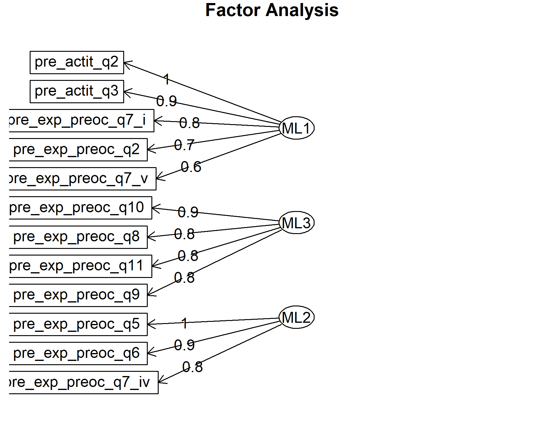
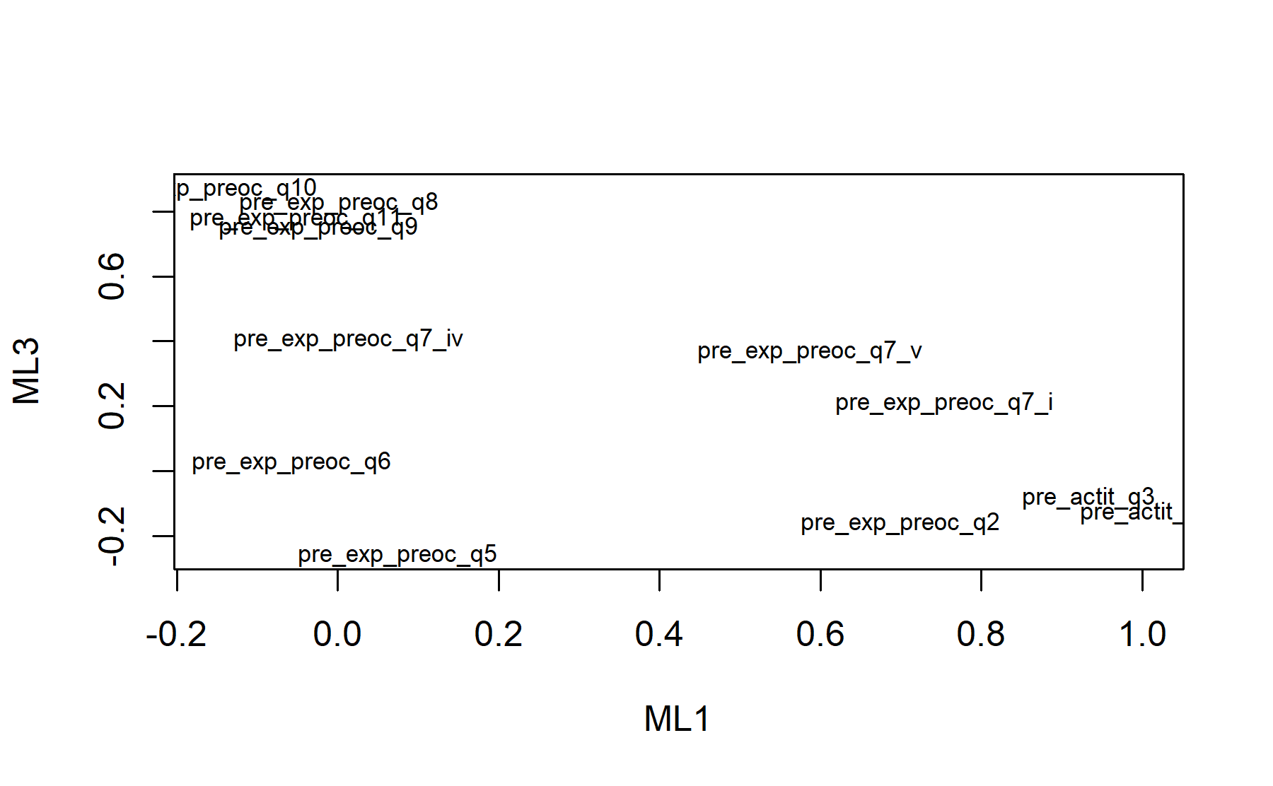
6.3.4.2 Expectations with the final set of items.
Now, the analysis with only expectations items excluding items Q1, Q4, Q7_ii, Q7_iii and Q3 is re-run.

The Barlett’s sphericity test is performed.
Thus, the p-value = 0 and the H0 is rejected confirming the utility of applying a factor analysis to this dataset.
Considering the fact that the Bartlett’s test usually rejects the H0 since the scenario of the null hypothesis is too extreme, the KMO analysis is studied to determine how well the data fit the factor analysis and how useful each item is.
## Kaiser-Meyer-Olkin factor adequacy
## Call: KMO(r = pre_test_Q_ExpConcern_facAn_4b_corr)
## Overall MSA =  0.64
## MSA for each item =
##    q2    q5    q6  q7_i q7_iv  q7_v    q8    q9   q10   q11
##  0.79  0.75  0.65  0.50  0.67  0.60  0.64  0.58  0.52  0.80
According to these results, all the items are above 0.5. Three items are below 0.6.
To explore the number of factors PCA is applied. Thus, the table with the PCA results is shown below:
| PC1 | PC2 | PC3 | PC4 | PC5 | PC6 | PC7 | PC8 | PC9 | PC10 | |
|---|---|---|---|---|---|---|---|---|---|---|
| Standard deviation | 1.9065 | 1.6936 | 1.0922 | 0.7671 | 0.7219 | 0.6701 | 0.5677 | 0.4381 | 0.3888 | 0.2831 |
| Proportion of Variance | 0.3635 | 0.2868 | 0.1193 | 0.0588 | 0.0521 | 0.0449 | 0.0322 | 0.0192 | 0.0151 | 0.0080 |
| Cumulative Proportion | 0.3635 | 0.6503 | 0.7696 | 0.8284 | 0.8805 | 0.9254 | 0.9577 | 0.9769 | 0.9920 | 1.0000 |
Then, the scree plot for this PCA analysis is displayed.
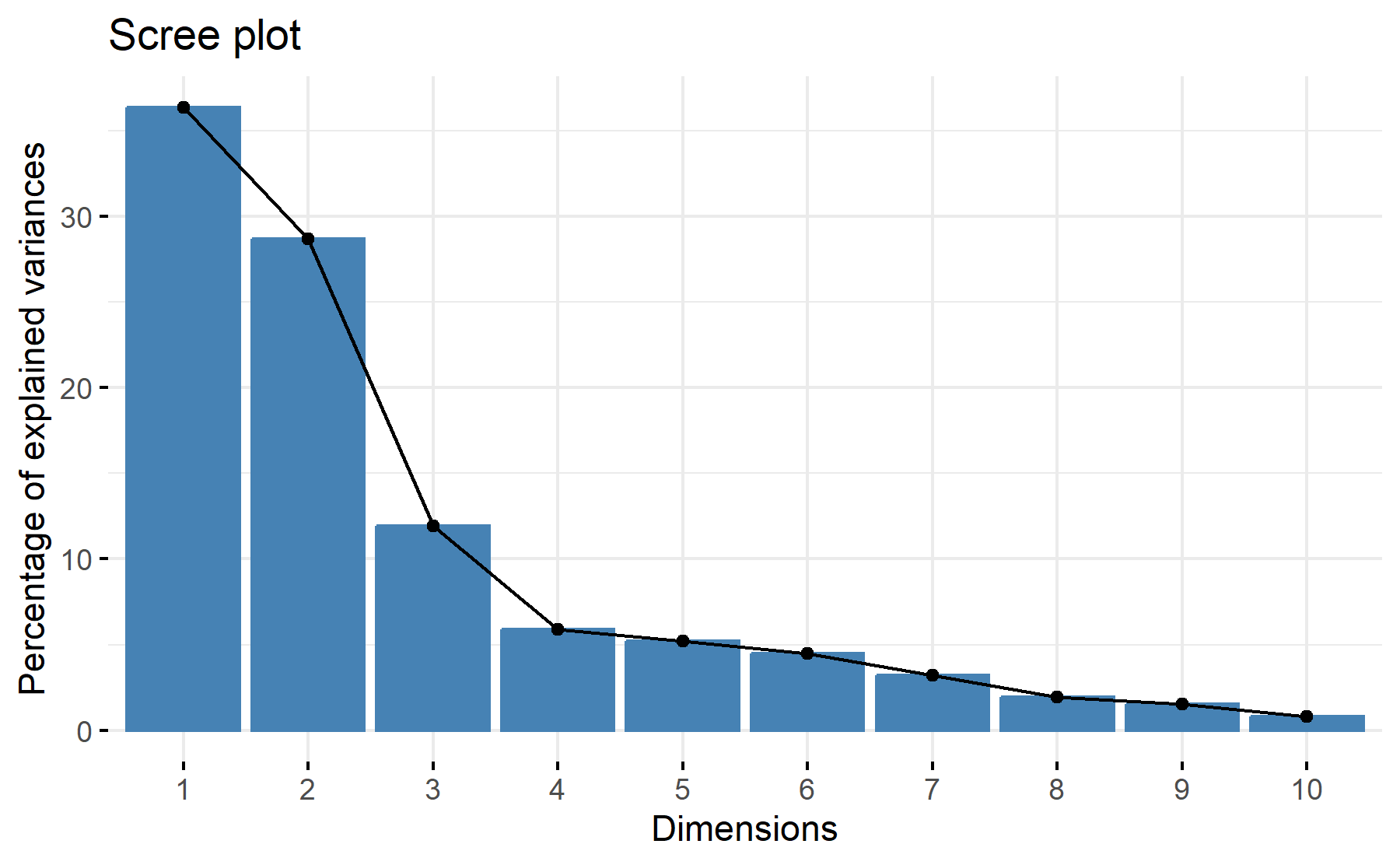 According to these results, 2-3 factors could be the best number. While the cumulative proportion for 3 components is 77%, for two is 65%; beside, two elbows can be identified, the first one after the second component, and the other one on the third component.
Then, another approach is implemented. With this strategy several analysis are combined and depict in the same figure. The tools implemented are: the Kaiser rule (which drops the components with eigenvalues < 1), the parallel analysis, and the usual scree test (plotuScree), the acceleration factor (which indicates where the elbow of the scree plot appears).
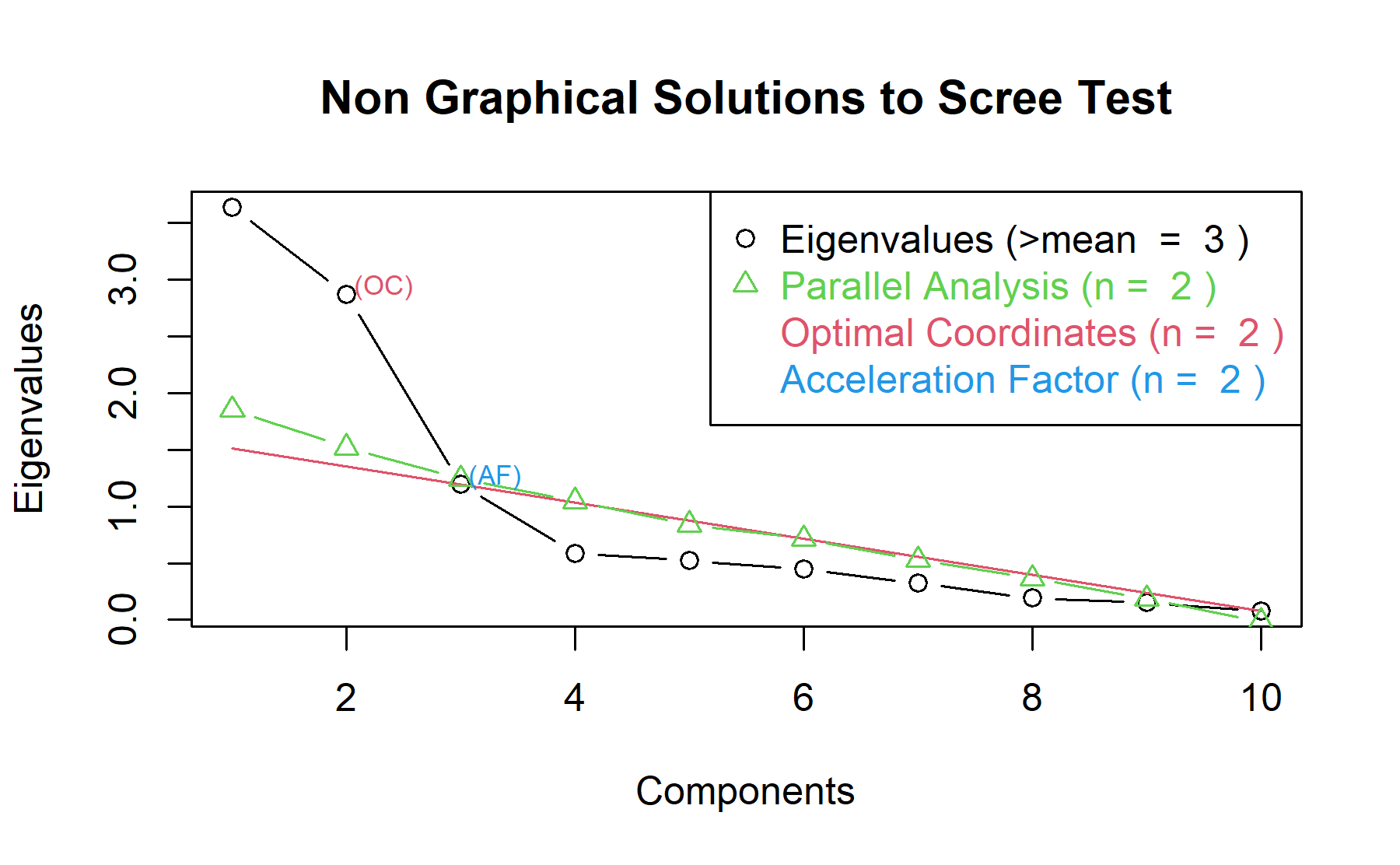 Therefore, considering two factors seem to be an adequate approach.
Running the factor analysis with 10 items, first the communalities are explored:
## Warning in cor.smooth(mat): Matrix was not positive definite, smoothing was
## done
## In factor.stats, I could not find the RMSEA upper bound . Sorry about that## pre_exp_preoc_q2 pre_exp_preoc_q5 pre_exp_preoc_q6 pre_exp_preoc_q7_i
## 0.4707 0.9267 0.8766 0.2682
## pre_exp_preoc_q7_iv pre_exp_preoc_q7_v pre_exp_preoc_q8 pre_exp_preoc_q9
## 0.9950 0.4067 0.6034 0.5948
## pre_exp_preoc_q10 pre_exp_preoc_q11
## 0.8194 0.7168Considering the values of the communalities, only Q7_i is below 0.3.
Then, the whole output is displayed.
## Factor Analysis using method =  ml
## Call: fa(r = pre_test_Q_ExpConcern_facAn_4b, nfactors = 2, rotate = "oblimin",
##     fm = "ml", cor = "poly")
## Standardized loadings (pattern matrix) based upon correlation matrix
##                       ML1   ML2   h2     u2 com
## pre_exp_preoc_q2     0.55 -0.46 0.47 0.5295 1.9
## pre_exp_preoc_q5     0.94       0.93 0.0733 1.2
## pre_exp_preoc_q6     0.93       0.88 0.1233 1.0
## pre_exp_preoc_q7_i   0.50       0.27 0.7328 1.2
## pre_exp_preoc_q7_iv  0.88  0.42 1.00 0.0049 1.4
## pre_exp_preoc_q7_v   0.63       0.41 0.5936 1.0
## pre_exp_preoc_q8           0.77 0.60 0.3969 1.0
## pre_exp_preoc_q9           0.73 0.59 0.4058 1.2
## pre_exp_preoc_q10          0.90 0.82 0.1805 1.1
## pre_exp_preoc_q11          0.83 0.72 0.2838 1.0
##
##                        ML1  ML2
## SS loadings           3.55 3.12
## Proportion Var        0.36 0.31
## Cumulative Var        0.36 0.67
## Proportion Explained  0.53 0.47
## Cumulative Proportion 0.53 1.00
##
##  With factor correlations of
##      ML1  ML2
## ML1 1.00 0.07
## ML2 0.07 1.00
##
## Mean item complexity =  1.2
## Test of the hypothesis that 2 factors are sufficient.
##
## df null model =  45  with the objective function =  50.32 with Chi Square =  947.6
## df of  the model are 26  and the objective function was  42.16
##
## The root mean square of the residuals (RMSR) is  0.12
## The df corrected root mean square of the residuals is  0.16
##
## The harmonic n.obs is  24 with the empirical chi square  32.22  with prob <  0.19
## The total n.obs was  24  with Likelihood Chi Square =  737.8  with prob <  8.3e-139
##
## Tucker Lewis Index of factoring reliability =  -0.475
## RMSEA index =  1.067  and the 90 % confidence intervals are  1.024 NA
## BIC =  655.2
## Fit based upon off diagonal values = 0.93
## Measures of factor score adequacy
##                                                    ML1  ML2
## Correlation of (regression) scores with factors   0.99 0.97
## Multiple R square of scores with factors          0.99 0.95
## Minimum correlation of possible factor scores     0.97 0.90
There are 2 factors:
* Q2, Q8, Q9, Q10, Q11, and Q7_iv
* Q5, Q6, Q7_i, Q7_iv, Q7_v, Q2.
No significant changes are detected when this case is excluded.
Finally, plots show the relationship between the items and the factors.