Chapter 9 Pre-test Questionnaire- Descriptive and exploratory analysis
9.1 Demographics
9.1.1 Descriptive Statistics
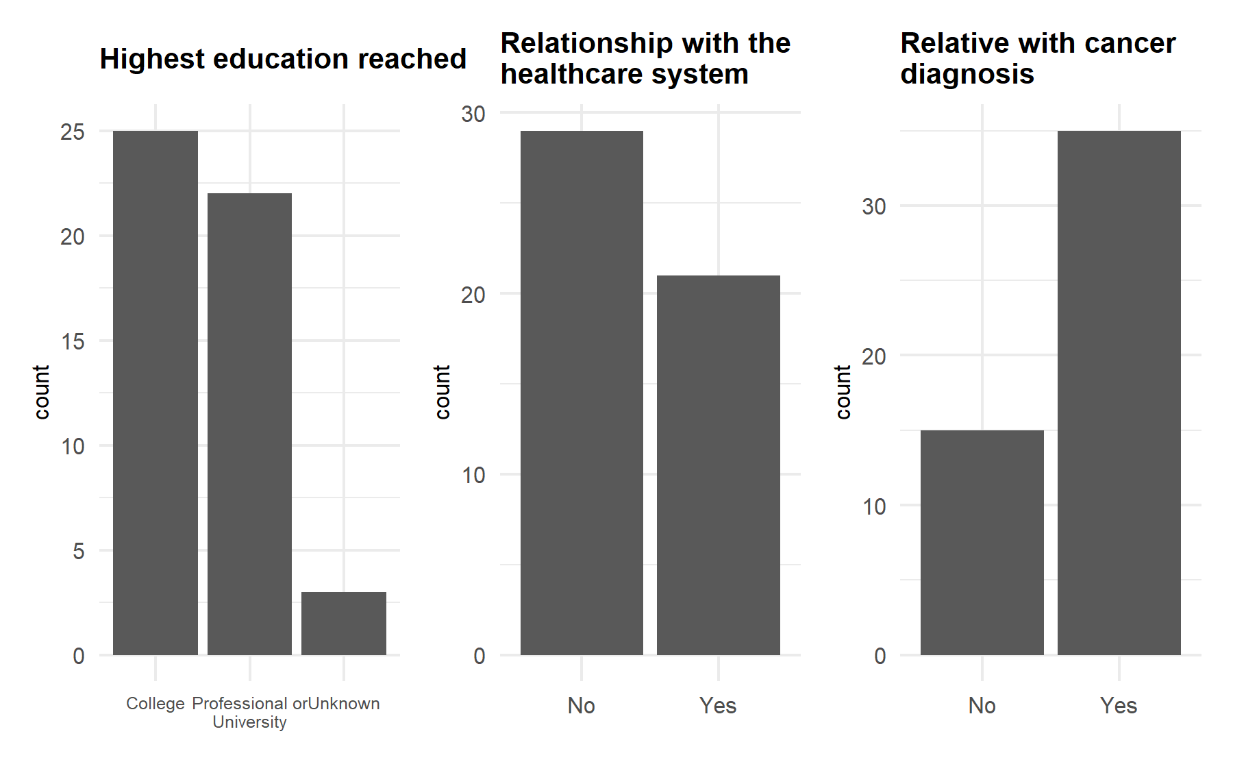
First, the demographics characteristics of the population included is analyzed.
| Overall | |
|---|---|
| n | 50 |
| Edad al diagnostico (mean (SD)) | 65.43 (8.82) |
| estado_civil.factor (%) | |
| A. Soltero y no vive en pareja | 4 ( 8.0) |
| B. Casado y/o vive en pareja | 44 (88.0) |
| D. Separado/Divorciado | 2 ( 4.0) |
| E. Viudo | 0 ( 0.0) |
| F. Otro (por favor especifique): | 0 ( 0.0) |
| G. Preferiría no decir | 0 ( 0.0) |
| ocupacion.factor (%) | |
| A. Trabajador en activo por cuenta propia | 2 ( 4.0) |
| B. Trabajador en activo por cuenta ajena | 10 (20.0) |
| C. Trabajador de baja/incapacidad debido a mi cáncer de próstata | 11 (22.0) |
| D. Jubilado o de baja/incapacidad previamente al diagnóstico | 27 (54.0) |
| formacion_academica.factor (%) | |
| A. Educación Primaria | 7 (14.3) |
| B. Educación Secundaria o Bachillerato | 14 (28.6) |
| C. Formación profesional | 7 (14.3) |
| D. Titulacion universitaria | 15 (30.6) |
| E. Otro (puede especificar): | 5 (10.2) |
| F. Preferiría no contestar | 1 ( 2.0) |
| exp_lab_salud.factor = B. No (%) | 47 (94.0) |
| fliar_salud.factor = B. No (%) | 29 (58.0) |
| fliar_cancer.factor = B. No (%) | 15 (30.0) |
| vivienda.factor (%) | |
| A. Vivo en una ciudad o area ámbito urbano | 41 (82.0) |
| B. Vivo en un pueblo | 9 (18.0) |
| C. Vivo en un area rural no urbanizada | 0 ( 0.0) |
9.2 Knowledge domain
In this domain there are 12 items. Out of these, 11 items were designed to chose one (or more) correct answers and the last item is about the source of knowledge without a correct or wrong answer and includes multiple information source options and patients could chose more than one. The target number of knowledge items to be included in the final version of this questionnaire is set in 5.
9.2.1 Descriptive statistics and sociodemographics comparison
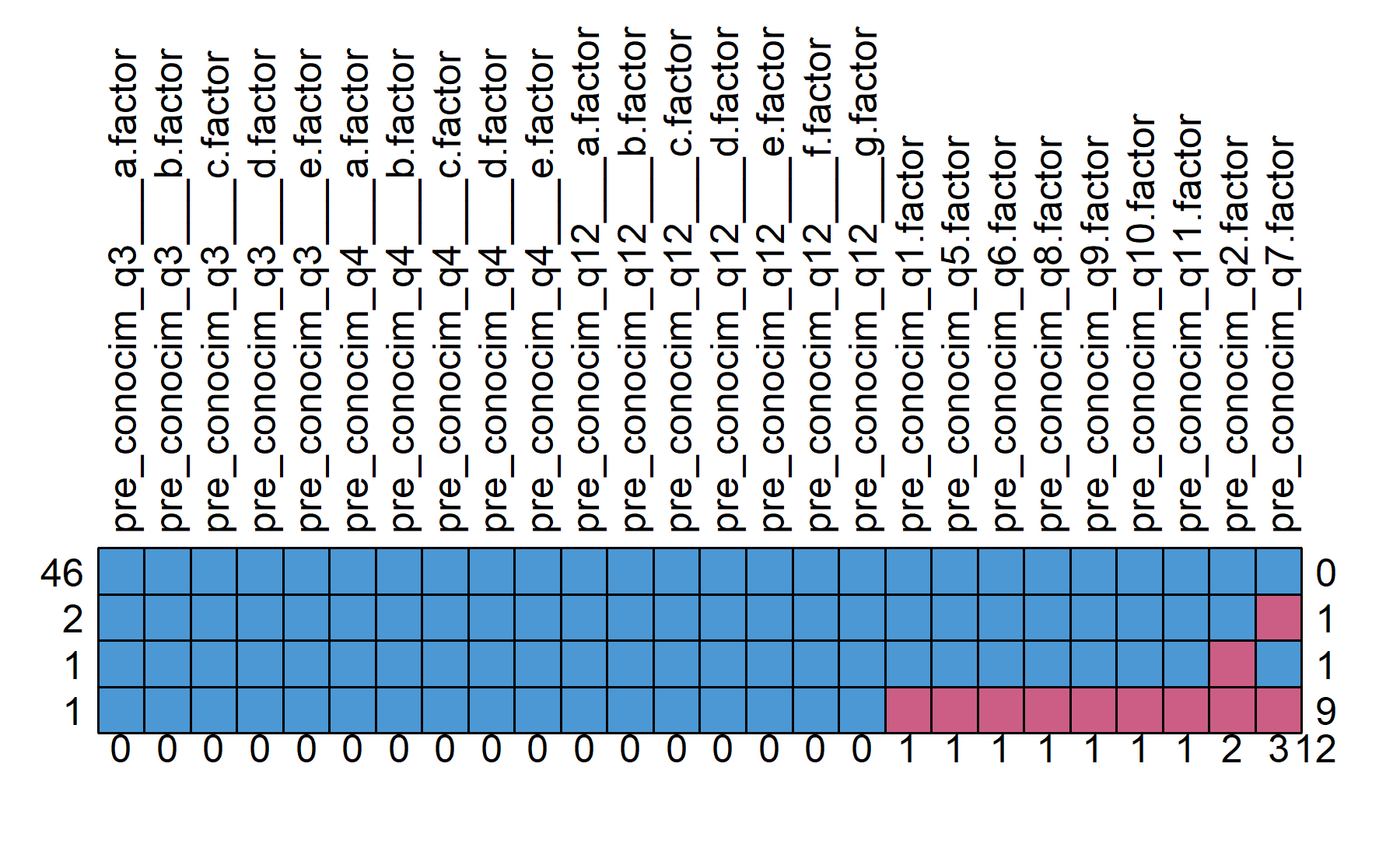
To start with the descriptive analysis, the missing data is explored.
##    pre_conocim_q3___a.factor pre_conocim_q3___b.factor
## 46                         1                         1
## 2                          1                         1
## 1                          1                         1
## 1                          1                         1
##                            0                         0
##    pre_conocim_q3___c.factor pre_conocim_q3___d.factor
## 46                         1                         1
## 2                          1                         1
## 1                          1                         1
## 1                          1                         1
##                            0                         0
##    pre_conocim_q3___e.factor pre_conocim_q4___a.factor
## 46                         1                         1
## 2                          1                         1
## 1                          1                         1
## 1                          1                         1
##                            0                         0
##    pre_conocim_q4___b.factor pre_conocim_q4___c.factor
## 46                         1                         1
## 2                          1                         1
## 1                          1                         1
## 1                          1                         1
##                            0                         0
##    pre_conocim_q4___d.factor pre_conocim_q4___e.factor
## 46                         1                         1
## 2                          1                         1
## 1                          1                         1
## 1                          1                         1
##                            0                         0
##    pre_conocim_q12___a.factor pre_conocim_q12___b.factor
## 46                          1                          1
## 2                           1                          1
## 1                           1                          1
## 1                           1                          1
##                             0                          0
##    pre_conocim_q12___c.factor pre_conocim_q12___d.factor
## 46                          1                          1
## 2                           1                          1
## 1                           1                          1
## 1                           1                          1
##                             0                          0
##    pre_conocim_q12___e.factor pre_conocim_q12___f.factor
## 46                          1                          1
## 2                           1                          1
## 1                           1                          1
## 1                           1                          1
##                             0                          0
##    pre_conocim_q12___g.factor pre_conocim_q1.factor pre_conocim_q5.factor
## 46                          1                     1                     1
## 2                           1                     1                     1
## 1                           1                     1                     1
## 1                           1                     0                     0
##                             0                     1                     1
##    pre_conocim_q6.factor pre_conocim_q8.factor pre_conocim_q9.factor
## 46                     1                     1                     1
## 2                      1                     1                     1
## 1                      1                     1                     1
## 1                      0                     0                     0
##                        1                     1                     1
##    pre_conocim_q10.factor pre_conocim_q11.factor pre_conocim_q2.factor
## 46                      1                      1                     1
## 2                       1                      1                     1
## 1                       1                      1                     0
## 1                       0                      0                     0
##                         1                      1                     2
##    pre_conocim_q7.factor
## 46                     1  0
## 2                      0  1
## 1                      1  1
## 1                      0  9
##                        3 12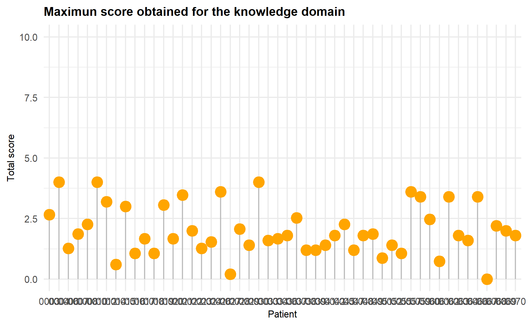
Knowledge is analyzed considering the sociodemographic variables. In this setting, three variables are compared: the health relationship, the highest education level acquired, and the presence of a relative with cancer. Plots and formal tests are performed.
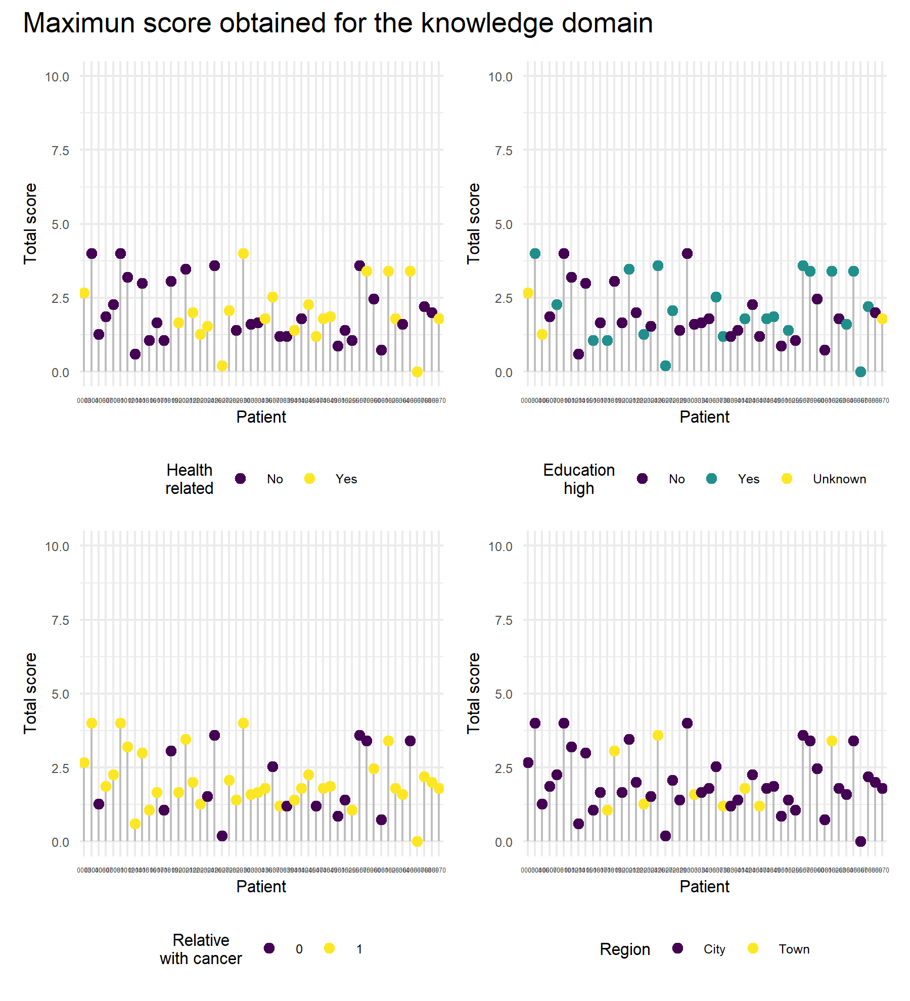
First, the educational level is analyzed.
## # A tibble: 3 × 11
## education_high n missing Minimun Maximun Mean DS Median FirstQ ThirdQ
## <fct> <int> <int> <dbl> <dbl> <dbl> <dbl> <dbl> <dbl> <dbl>
## 1 No 25 0 0.6 4 1.92 0.918 1.67 1.4 2.27
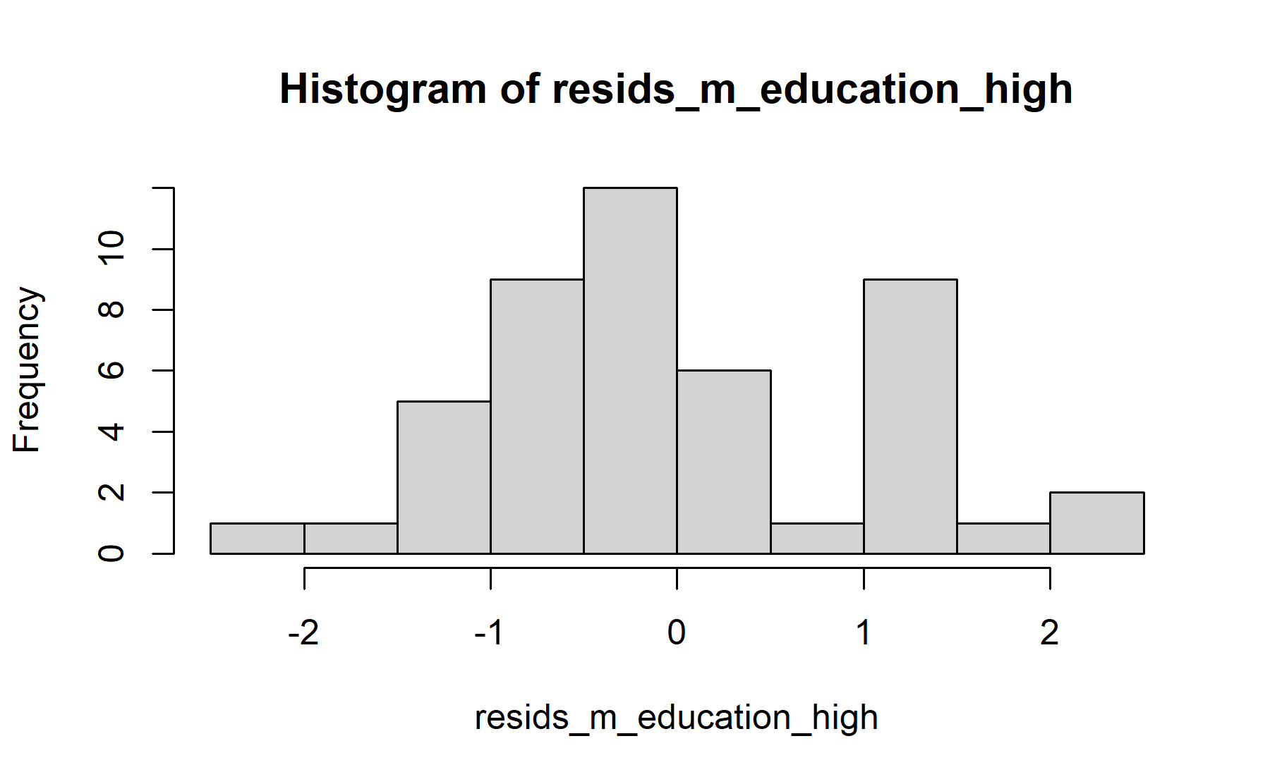
## 2 Yes 22 0 0 4 2.15 1.15 1.97 1.3 3.4
## 3 Unknown 3 0 1.27 2.67 1.91 0.707 1.8 1.53 2.23
## # ℹ 1 more variable: IQR <dbl>##
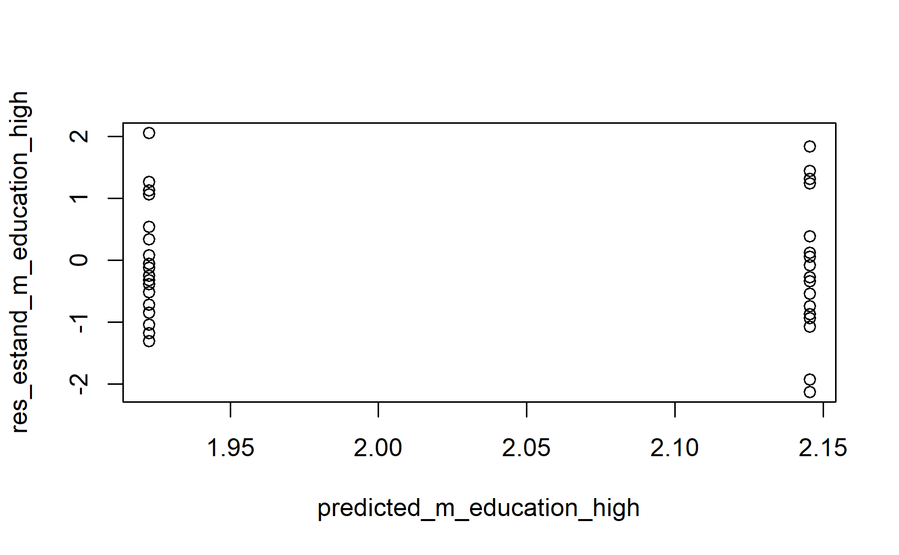
## Shapiro-Wilk normality test
##
## data: resids_m_education_high
## W = 0.96, p-value = 0.08
## Levene's Test for Homogeneity of Variance (center = median)
##       Df F value Pr(>F)
## group  2    1.38   0.26
##       47
##
## Two Sample t-test
##
## data: knowg_correct_totalsum by education_high
## t = -0.74, df = 45, p-value = 0.5
## alternative hypothesis: true difference in means between group No and group Yes is not equal to 0
## 95 percent confidence interval:
## -0.8316 0.3860
## sample estimates:
## mean in group No mean in group Yes
## 1.923 2.145There is not significant difference between scores from both groups with different educational levels, the mean score for the knowledge questions in the group with the highest educational level was 2.15 (sd 1.15), and it was 1.92 (sd 0.92) in the other group (p=0.5).
First, the relationship with health is analyzed.
## # A tibble: 2 × 11
##   health_related     n missing Minimun Maximun  Mean    DS Median FirstQ ThirdQ
##   <chr>          <int>   <int>   <dbl>   <dbl> <dbl> <dbl>  <dbl>  <dbl>  <dbl>
## 1 No                29       0     0.6       4  2.03 1.03    1.67   1.2    3
## 2 Yes               21       0     0         4  2.00 0.999   1.8    1.53   2.53
## # ℹ 1 more variable: IQR <dbl>
##
## Shapiro-Wilk normality test
##
## data: resids_m_health_related
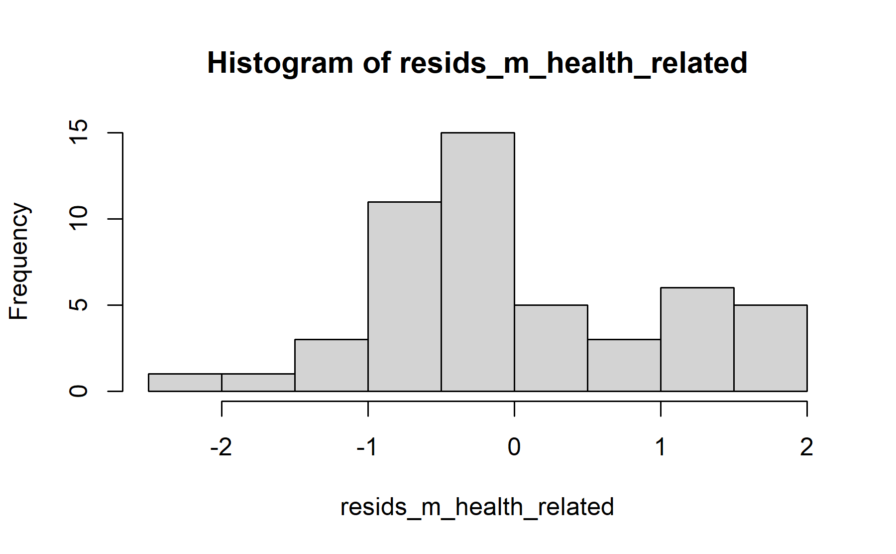
## W = 0.95, p-value = 0.05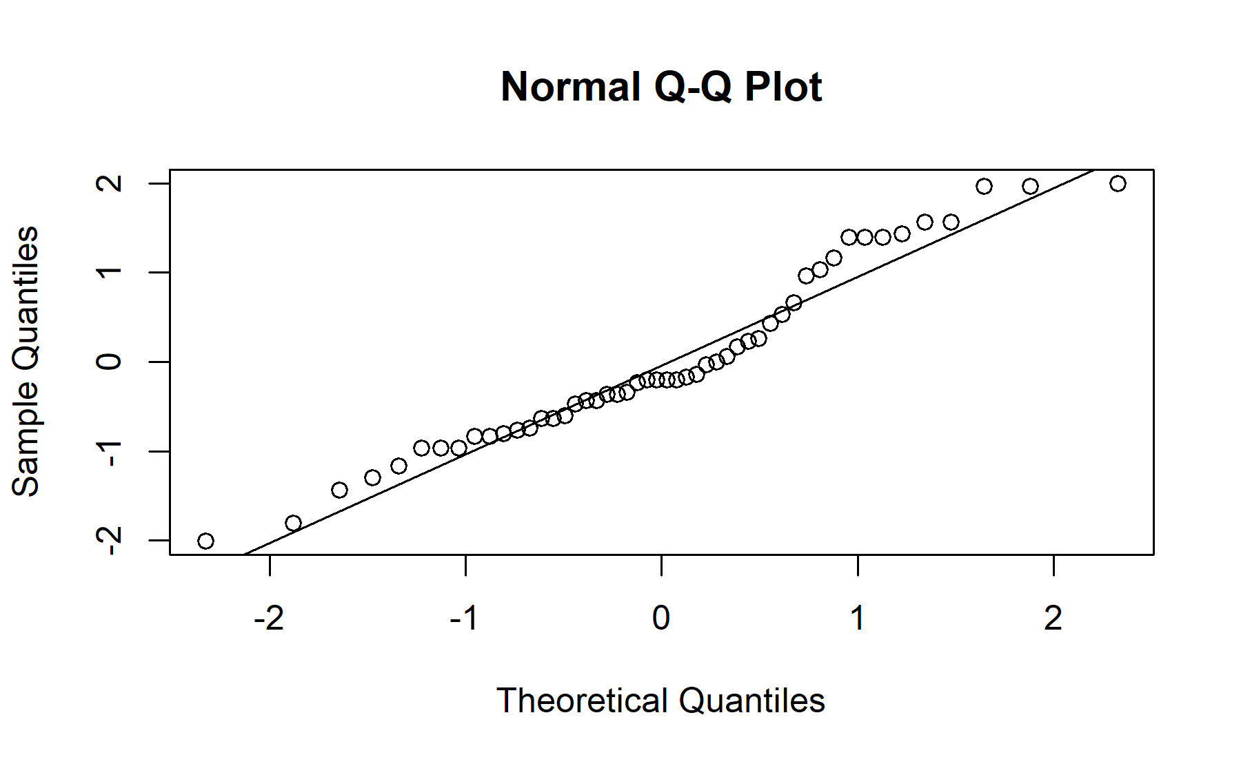
## Levene's Test for Homogeneity of Variance (center = median)
##       Df F value Pr(>F)
## group  1    0.29   0.59
##       48
##
## Two Sample t-test
##
## data: pre_test_Q_Conocim$knowg_correct_totalsum by pre_test_Q_Conocim$health_related
## t = 0.099, df = 48, p-value = 0.9
## alternative hypothesis: true difference in means between group No and group Yes is not equal to 0
## 95 percent confidence interval:
## -0.5573 0.6153
## sample estimates:
## mean in group No mean in group Yes
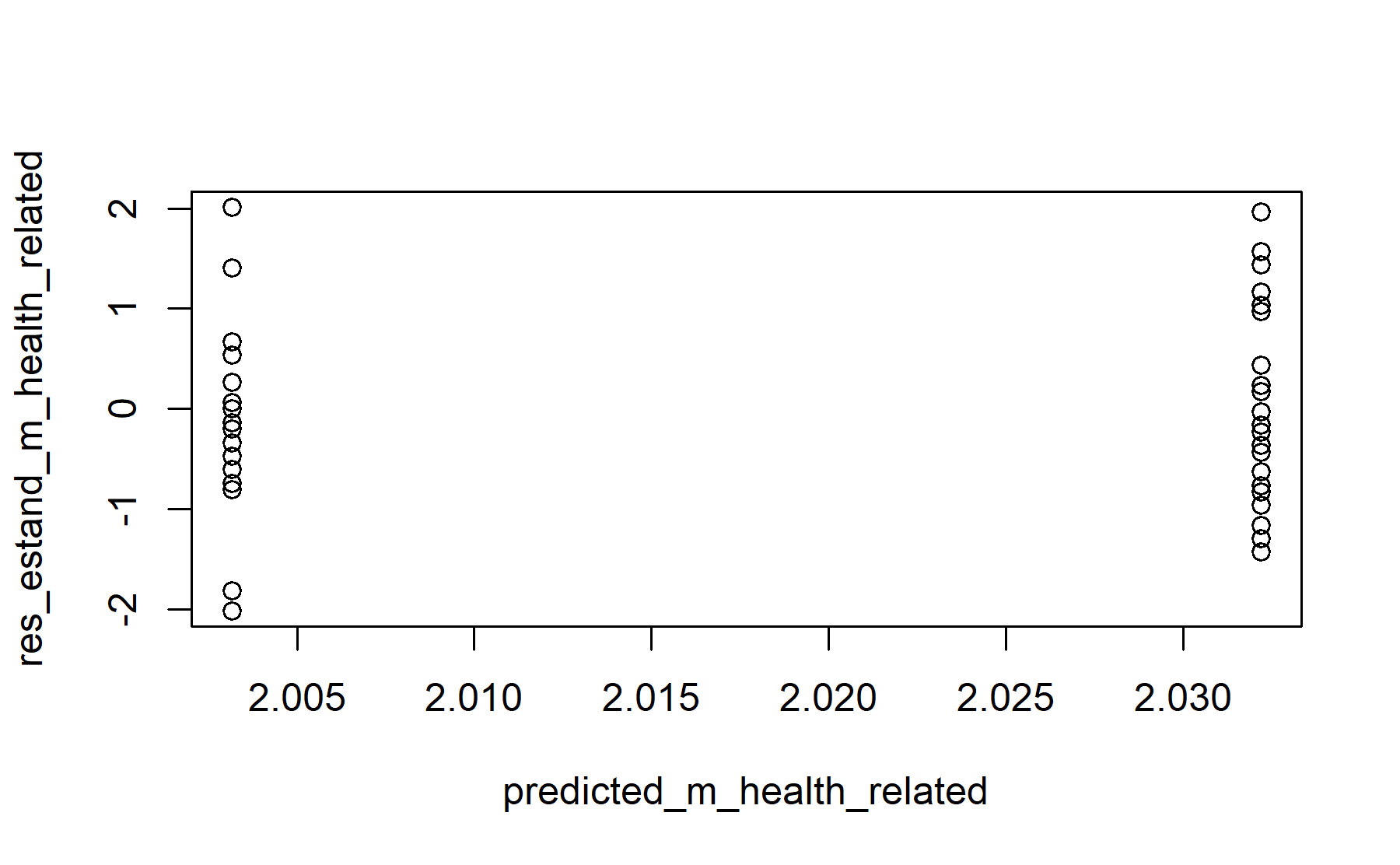
## 2.032 2.003No difference was seen between scores from both groups of health relationship, the mean score for the knowledge questions in the group related with health was 2.03 (sd 1.00), and it was 2.00 (sd 1.03) in the other group (p=0.9).
Then, the influence of a relative with cancer is analyzed.
## # A tibble: 2 × 11
##   fliar_cancer     n missing Minimun Maximun  Mean    DS Median FirstQ ThirdQ
##   <labelled>   <int>   <int>   <dbl>   <dbl> <dbl> <dbl>  <dbl>  <dbl>  <dbl>
## 1 0               15       0     0.2     3.6  1.94 1.19     1.4   1.13   3.23
## 2 1               35       0     0       4    2.06 0.936    1.8   1.6    2.37
## # ℹ 1 more variable: IQR <dbl>
##
## Shapiro-Wilk normality test
##
## data: resids_m_fliar_cancer
## W = 0.94, p-value = 0.02
## Levene's Test for Homogeneity of Variance (center = median)
##       Df F value Pr(>F)
## group  1    1.79   0.19
##       48
##
## Two Sample t-test
##
## data: pre_test_Q_Conocim$knowg_correct_totalsum by pre_test_Q_Conocim$fliar_cancer
## t = -0.37, df = 48, p-value = 0.7
## alternative hypothesis: true difference in means between group 0 and group 1 is not equal to 0
## 95 percent confidence interval:
## -0.7481 0.5132
## sample estimates:
## mean in group 0 mean in group 1
## 1.938 2.055The same score was observed for both groups, without any significant difference, mean score in the group that has relatives with cancer was 2.06 (sd 0.94), and 1.94 (sd 1.19) in the other group (p=0.7).
Finally, the region where the patient lives is considered.
## # A tibble: 2 × 11
##   vivienda_cat     n missing Minimun Maximun  Mean    DS Median FirstQ ThirdQ
##   <fct>        <int>   <int>   <dbl>   <dbl> <dbl> <dbl>  <dbl>  <dbl>  <dbl>
## 1 City            41       0    0        4    2.02  1.01    1.8    1.4   2.53
## 2 Town             9       0    1.07     3.6  2.02  1.03    1.6    1.2   3.07
## # ℹ 1 more variable: IQR <dbl>
##
## Shapiro-Wilk normality test
##
## data: resids_m_vivienda
## W = 0.95, p-value = 0.04
## Levene's Test for Homogeneity of Variance (center = median)
##       Df F value Pr(>F)
## group  1    0.01   0.93
##       48
##
## Two Sample t-test
##
## data: pre_test_Q_Conocim$knowg_correct_totalsum by pre_test_Q_Conocim$vivienda_cat
## t = -0.0072, df = 48, p-value = 1
## alternative hypothesis: true difference in means between group City and group Town is not equal to 0
## 95 percent confidence interval:
## -0.7560 0.7506
## sample estimates:
## mean in group City mean in group Town
## 2.020 2.022The same score was observed for both groups, without any significant difference, mean score in the group that lives in the city was 2.02 (sd 1.01), and 2.02 (sd 1.03) for those who lives in a town (p=1).
Results according to the type of job or if they are retired are describe considering the knowledge score.
## # A tibble: 4 × 11
## ocupacion_cat n missing Minimun Maximun Mean DS Median FirstQ ThirdQ
## <chr> <int> <int> <dbl> <dbl> <dbl> <dbl> <dbl> <dbl> <dbl>
## 1 On sick leave 11 0 1.2 3.6 2.34 0.934 2 1.6 3.3
## 2 Retired 27 0 0 4 1.92 1.05 1.67 1.23 2.57
## 3 Working, emplo… 10 0 0.733 4 2.05 1.06 1.83 1.25 2.27
## 4 Working, self-… 2 0 1.4 1.6 1.5 0.141 1.5 1.45 1.55
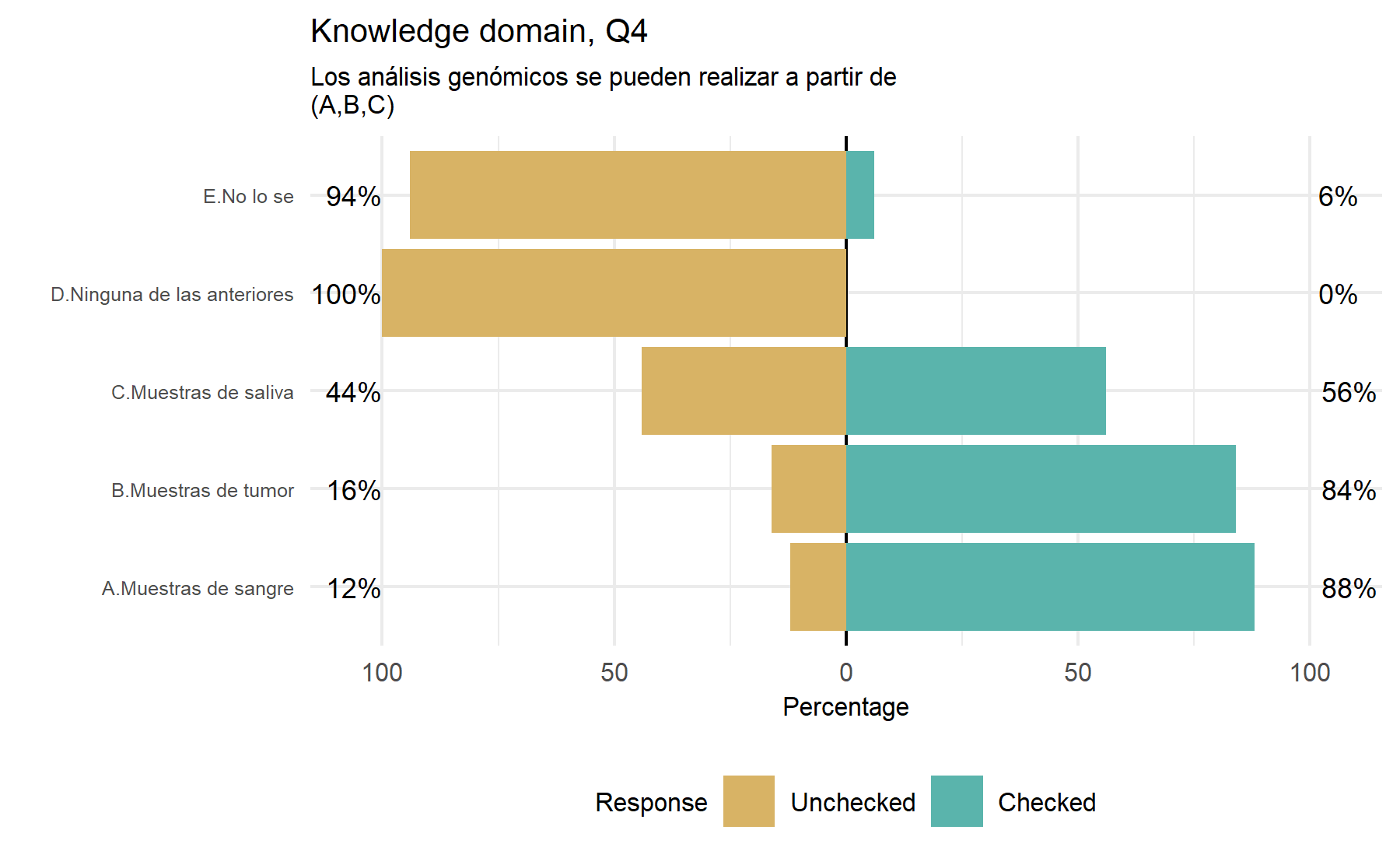
## # ℹ 1 more variable: IQR <dbl>Finally, according to the last item asking about the source of information, the results are shown below.
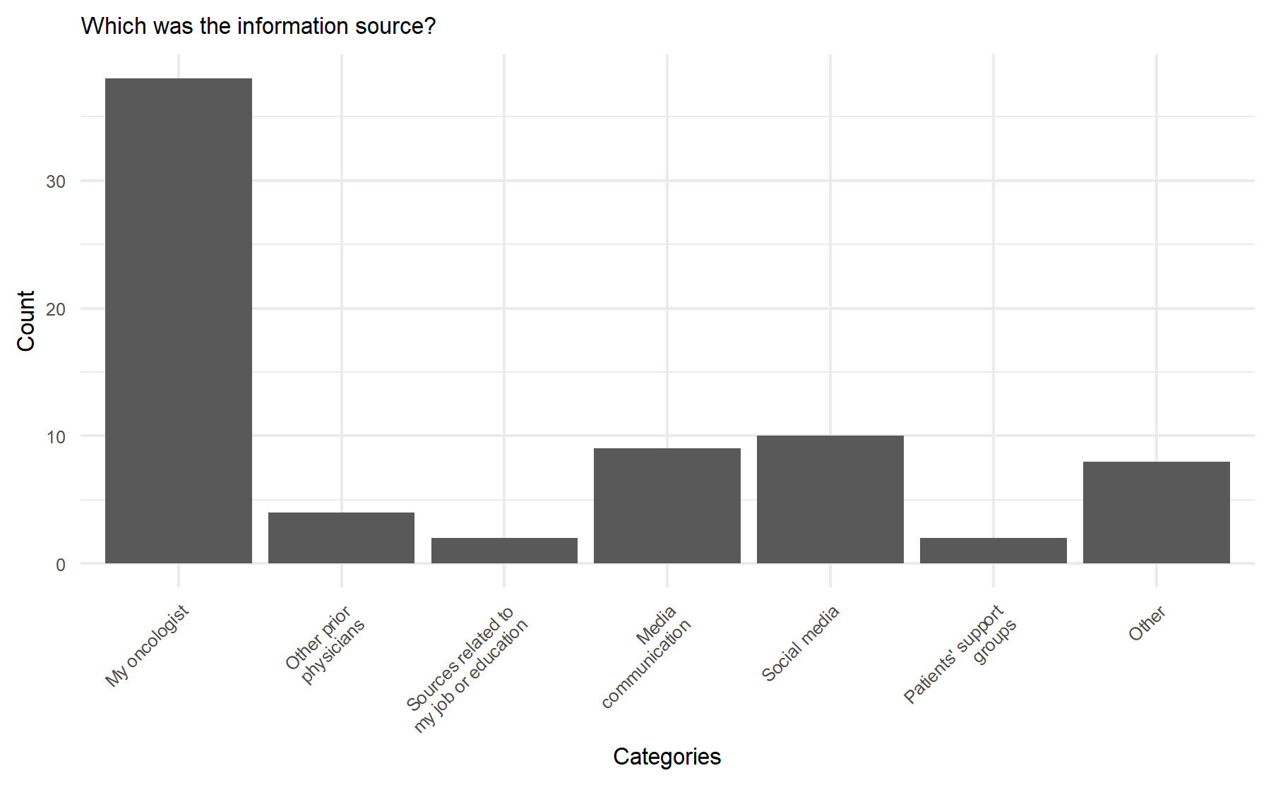 To note, in this item, patients could select more than one option. However, the results demonstrate that the most frequent source was their oncologist.
9.2.1.1 Analysis of each question across the patients.
Now, results for each question across all the patients are shown. Questions with binary responses are displayed together, then the remaining two questions with multiple options.
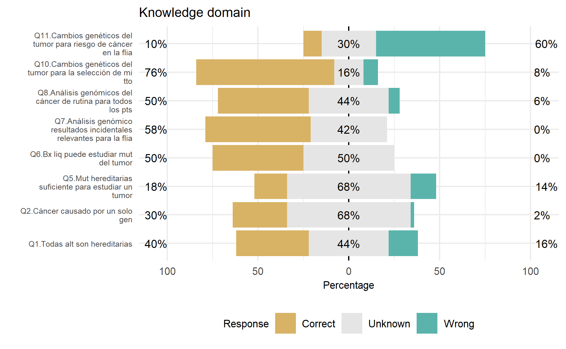
From the analysis of this set of 8 questions, some conclusions can be extracted evaluating the frequency of correct and wrong answers. Similar to what was found before, there is a high frequency of answers tagged as unknown. While the Q10 has mostly correct answers, Q11 has the lowest percentage of correct ones. Items 6 and 7 do not show wrong responses. The questions with more useful variability are Q1, Q5, Q8, and 11. Q7 could be meaningful for the tool itself.
Potential questions: Q1, Q5, Q8, Q11, and Q7.
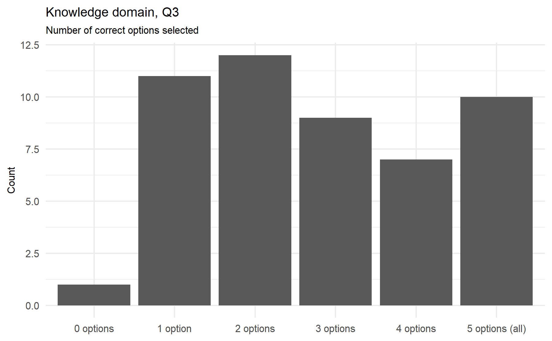
After this analysis of the variability of the answers a first conclusion can be drawn. It is desired to select questions with a lower proportion of unknown answers and with a similar proportion of correct and incorrect options selected. A higher proportion of unknown answers possibly reflects a hard-to-know or understand question, and this fact pinpoints a problematic item. On the other hand, a unknowns would reflect an area of uncertainty and room to add some type of intervention such as an educational intervention. A similar proportion between correct and incorrect answers implies a high variability between subjects; thus, it is expected that this item could gather a higher amount of information. Therefore, a score (from 1 to 10) is assigned to each item considering these characteristics. This score represents the importance order of each item with regard to the total (n=10).
Then, in a second stage, a measure of correlation between each item and the total score is explore. An Spearman correlation is determined for the two items with several options (Q3 and Q4). For the remaining 8 questions with correct/incorrect results cannot be possible to compute a correlation coefficient. Thus, for these items a visual strategy is explore.
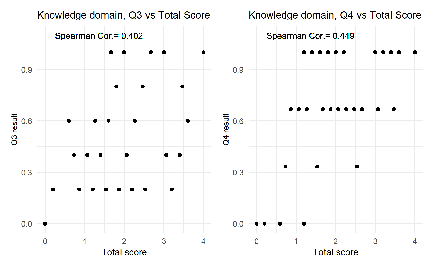
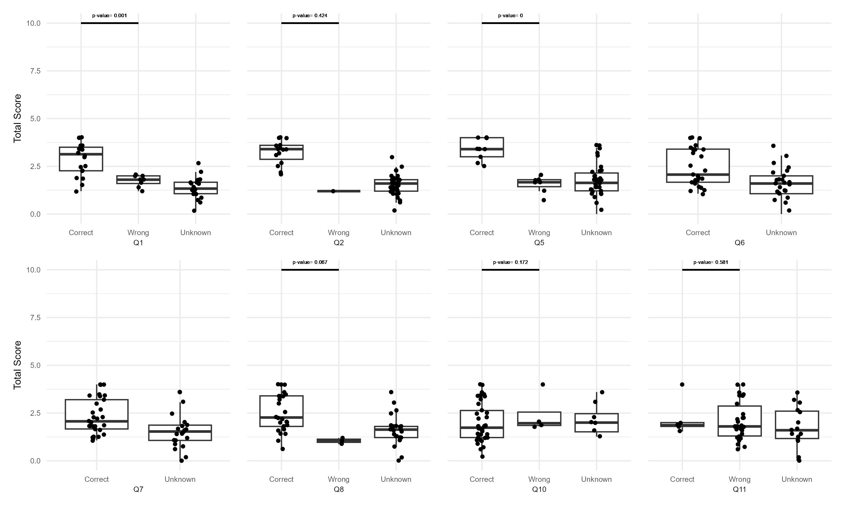
After these analyses the results obtained are summarize in the following table (organized by the variability factor):
| items | variability | Median_pvalue | Sp_correlation |
|---|---|---|---|
| Q1 | 1 | 3.1 (p=0.001) | NA |
| Q5 | 2 | 3.4 (p=0) | NA |
| Q3 | 3 | NA | 0.402 |
| Q11 | 4 | 1.9 (p=0.581) | NA |
| Q2 | 5 | 3.4 (p=0.424) | NA |
| Q8 | 6 | 2.3 (p=0.067) | NA |
| Q7 | 7 | NA | NA |
| Q4 | 8 | NA | 0.449 |
| Q10 | 9 | 1.7 (p=0.172) | NA |
| Q6 | 10 | NA | NA |
9.2.2 Global conclusions about knowledge domain
Q11 and Q10 seem to be the less useful items. Then, questions Q1, and Q5, followed by Q8 have the highest association between correct answers and a higher total score. While Q2 does not show statistically significant difference, there is an increase between correct and unknown answers; this effect is less clear for Q6 and Q7. Then, Q4 and Q3 have a moderate correlation with the total score.
Comparing these results with those from the VHIO cohort, while trends are similar in the VHIO group there are more numerical differences for items 10 and 11. However, for these two variables there was not significant difference in VHIO cohort neither. Additionally, item 6 and 7 in this study do not have wrong answers (only correct and unknown). Items Q3 and Q4 were more relevant in the VHIO analysis, which can be explained by the design of the study in each patient population. Considering a wider approach, the HOPE study could be more accurate to represent the general population landscape. Therefore, in this study the Q4 asking about the type of sample in which a genomic testing can be performed seems to be less useful. Then, Q6 and Q7 were found relevant in VHIO while in HOPE their role is less clear; principally, because they do not have wrong answers.
Conclusion: Q1, Q5, and Q8 were relevant in both cohorts. Then, Q3 can add valuable information and granularity. Finally, Q7 is relevant due to the fact that include incedental findings.
9.3 Expectations and concerns domain
In this setting, expectations and concerns are studied. In this domain there are 11 questions, but one (the seventh) has 5 items. Thus, there are a total of 15 items in this domain. These items can be divided into expectations, from 1 to 7.v., and concerns, from 8 to 11. All of them with a likert scale with 5 levels: Totalmente en desacuerdo, Algo en desacuerdo, Ni de acuerdo ni en desacuerdo, Algo de acuerdo, Totalmente de acuerdo.
9.3.1 Visualizing items and responses
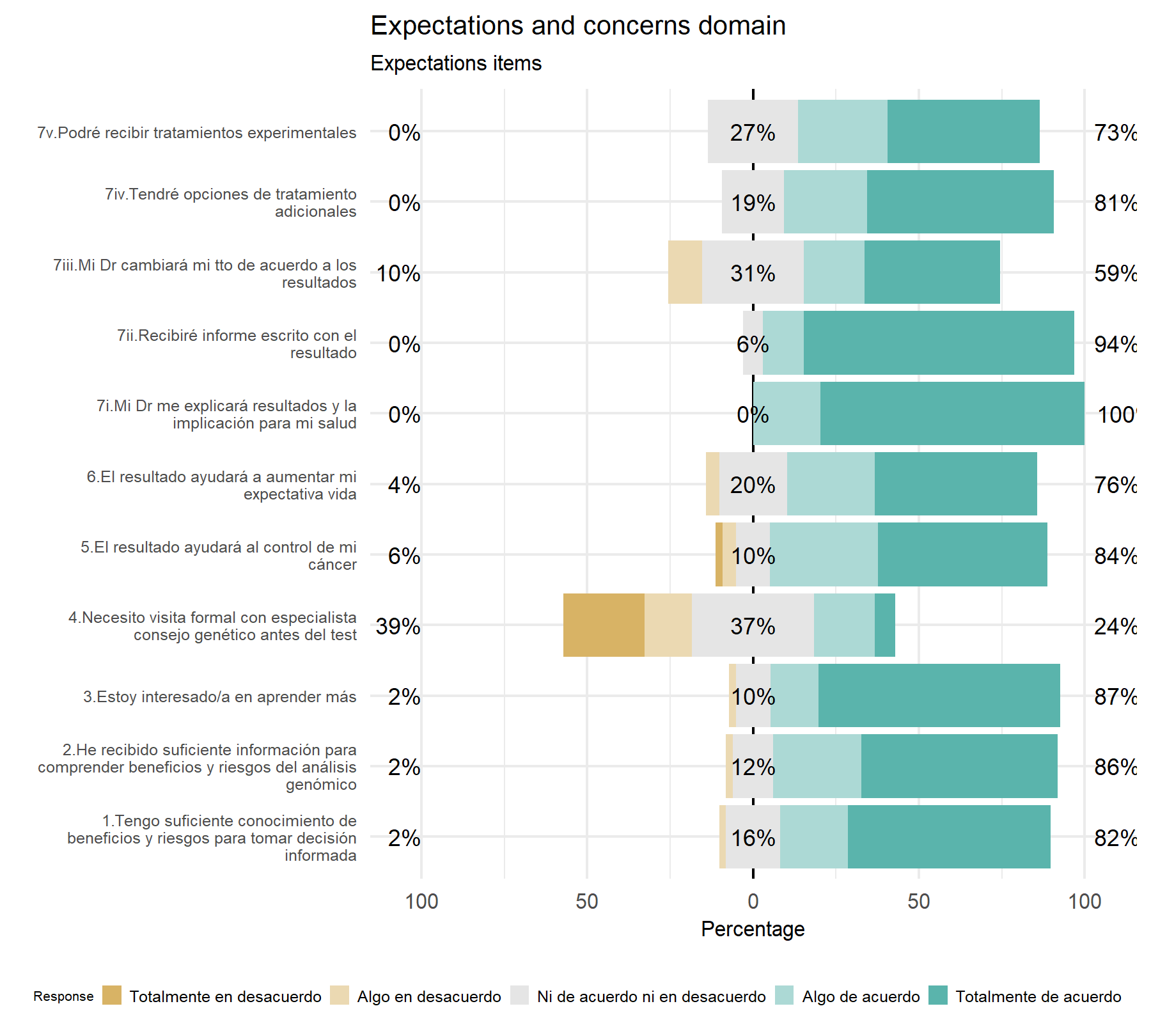
From the first visual analysis, all items have a wide majority of agreement answers, with a higher percentage of totally agree answers. Then, items with less variability are 7.ii and 7.i. Those with more variability are item 4, with an inverted design, have 16% with totally disagree and 40% with totally agree answers; followed by item 6. Then, there are two groups, one including item 5 and 7.iv with a higher number of agreement (with a relevant percentage of partially agreement), between 12-15% neither agreement nor disagreement, and the highest percentage of disagreement. The second group includes item 3, 2, 1, and 7.v with a similar distribution of answers (65-75% agreement, 25-30% of neither agreement nor disagreement, and a lower percentage of disagreement). It is important to highlight that item 2 and 1 are widely overlapped, thus, it is expected to chose one of them. Additionally, item 7.iv has one of the highest percentage of totally disagreement but also one of the highest levels of totally agreement.
For these two groups of items, expectations and concerns, proportions of answers seems to be similar regarding previous VHIO study. A more formal comparison could be performed.
As second exploratory approach analysis, the difficulty and discrimination capacity is evaluate for each of these items.
## Scale for fill is already present.
## Adding another scale for fill, which will replace the existing scale.
## Scale for colour is already present.
## Adding another scale for colour, which will replace the existing scale.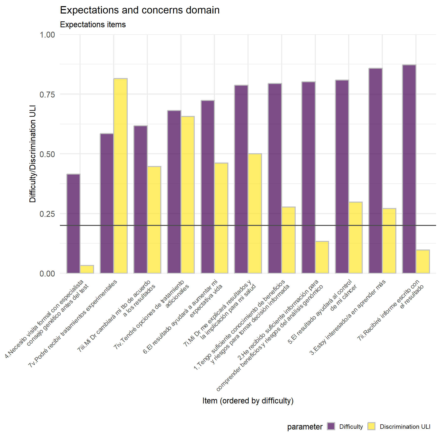
Regarding discrimination there is several differences between both cohorts. In this cohort, the items with the highest discrimination score are Q7.v, Q7.iv, and Q7.i, followed by Q7.iii. Then, Q4, Q2, and Q7.ii felt below the threshold. Considering the previous cohort, the highest score was for Q7.v as well, but then none except Q4 were below the threshold and Q2 was the second in terms of discrimination capacity.
## Scale for fill is already present.
## Adding another scale for fill, which will replace the existing scale.
## Scale for colour is already present.
## Adding another scale for colour, which will replace the existing scale.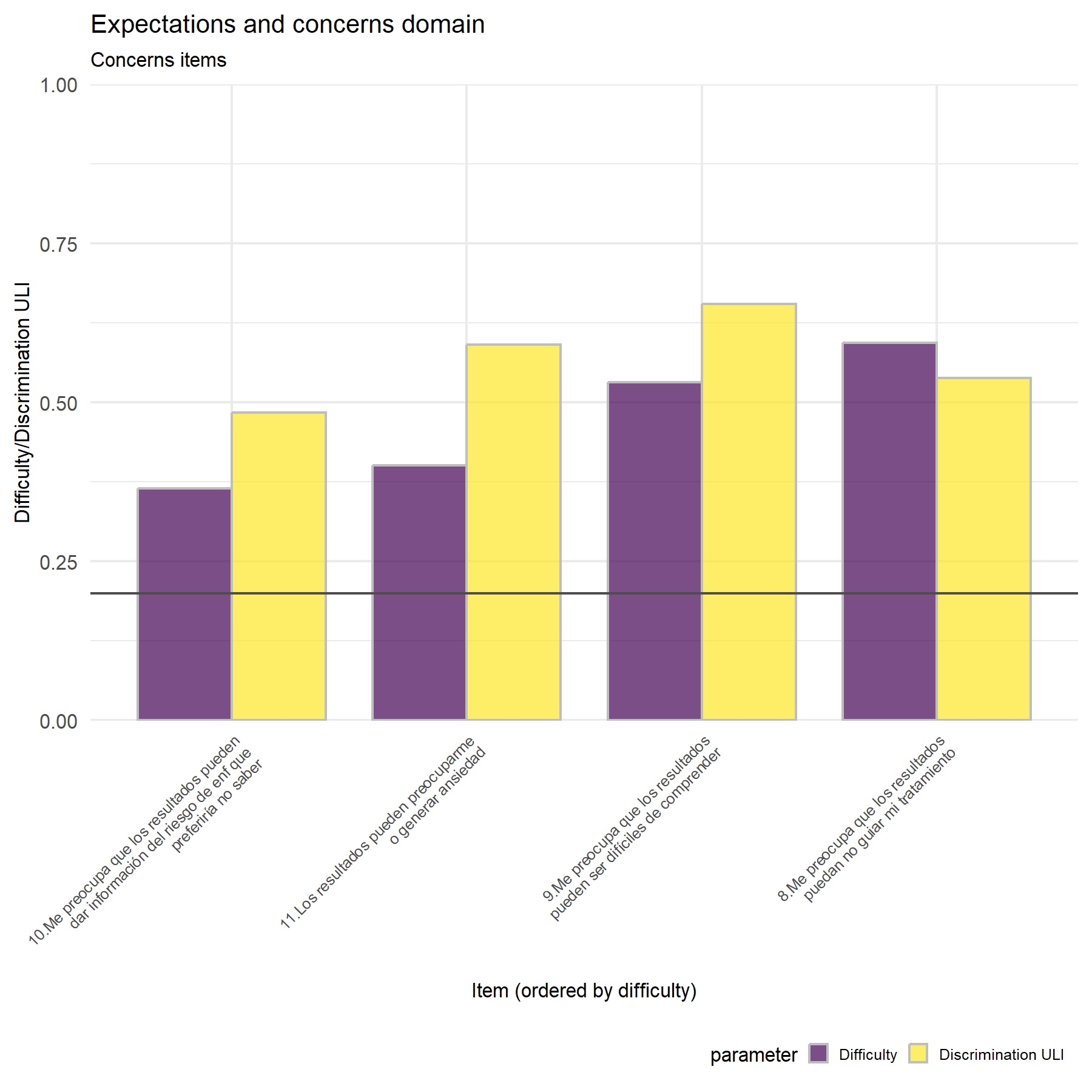
Discrimination is similar between studies when concerns items are analyzed.
Partial conclusion:
Expectations.
Variability- Highest variability: Q4, and Q6. Then, similarly to the VHIO cohort, there is two groups. One composed by Q5 and Q7.iv and 3, 2, 1, and 7.v. It is important to note that item 1 and 2 are equivalent, only one will be selected. Moreover, Q7.iv has one of the highest percentage of totally disagreement but also one of the highest levels of totally agreement.
Lowest variability: 7.ii and 7.i.
Discrimination- Highest discrimination: 7.v, 7.iv, 7.i, and 6.
Lowest discrimination: item 4, 2, 7.ii, followed by 1 and 3.
summary-
The best five elements are: Q6, Q7.v, Q7.iv, Q5, then Q2 and Q7.i.
The worst two: Q4 and Q7.ii.
Even when Q7.iii could not be useful from this perspective, could be key when answers were compared before and after the genomic testing.
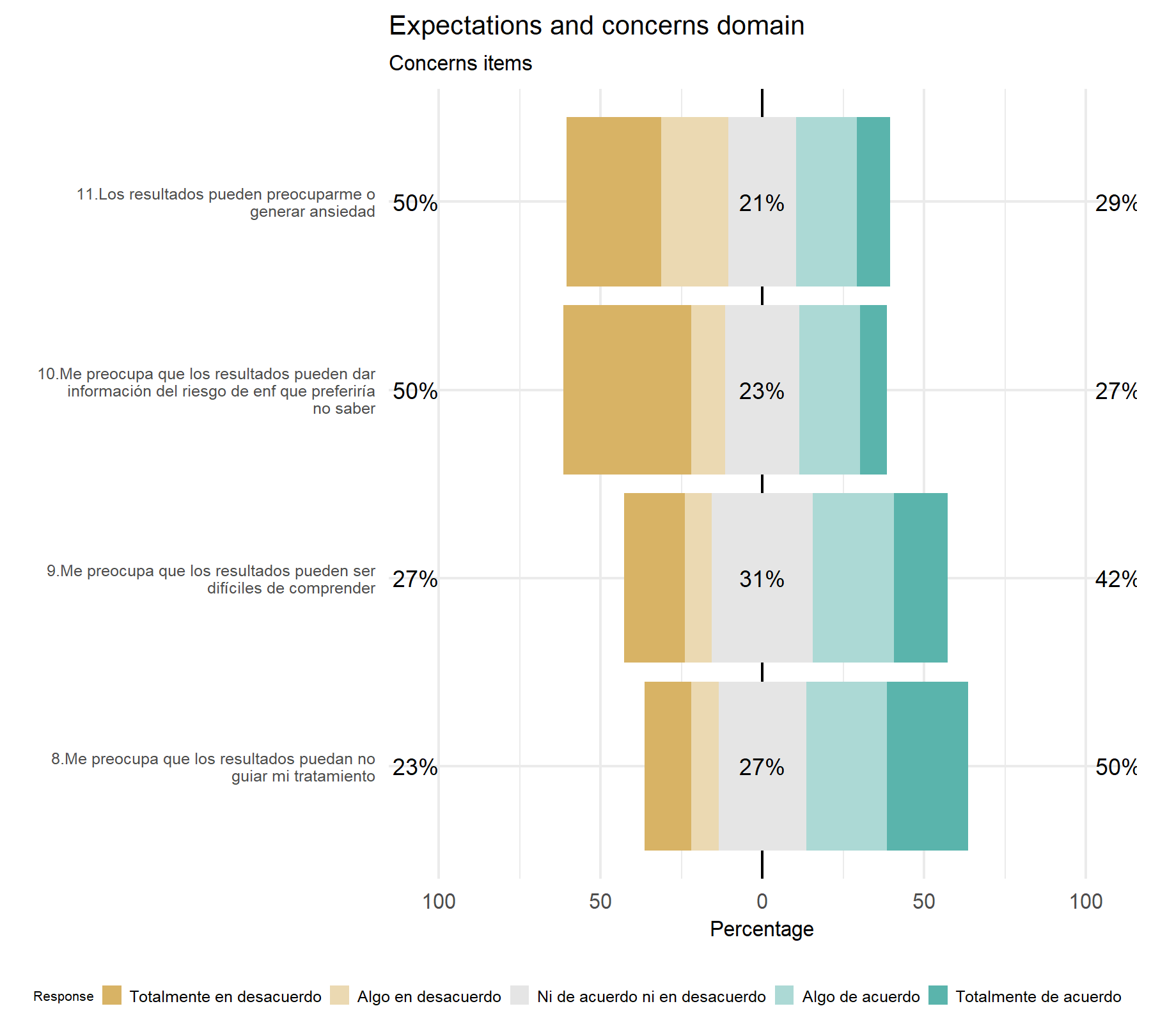
Concerns.
Variability- There is no clear variability.
Discrimination- There is not clear discrimination.
9.3.2 Evaluating the reliability of questions (Cronbach’s α and Omega)
The Cronbach’s α and the Guttman’s lambda_6 (G6) are calculated for expectations and later for concerns.
9.3.2.1 Expectations
Regarding expectations items, the number 4 will be inverted.
First, analyzing the reliability of the whole subset of items, i.e., the consistency of the expectations section several measurements are display: the Cronbach’s α, with its IC, and the omega (ω) coefficient.
##
##    95% confidence boundaries (Feldt)
##  lower alpha upper
##   0.56   0.7  0.81
##
## Information about this analysis:
##
## Dataframe: pre_test_Q_Expectations_values[, 2:12]
## Items: all
## Observations: 47
## Positive correlations: 43 out of 55 (78%)
##
## Estimates assuming interval level:
##
## Omega (total): 0.79
## Omega (hierarchical): 0.44
## Revelle's omega (total): 0.79
## Greatest Lower Bound (GLB): NA
## Coefficient H: 0.9
## Coefficient alpha: 0.69
##
## (Estimates assuming ordinal level not computed, as the polychoric correlation matrix has missing values.)
##
## Note: the normal point estimate and confidence interval for omega are based on the procedure suggested by Dunn, Baguley & Brunsden (2013) using the MBESS function ci.reliability, whereas the psych package point estimate was suggested in Revelle & Zinbarg (2008). See the help ('?scaleStructure') for more information.Here, both, alpha and omega are lower than in the VHIO cohort.
Then, in order to inspect the role of each item, the r.cor and the Guttman’s Lambda 6 (G6) are explored.
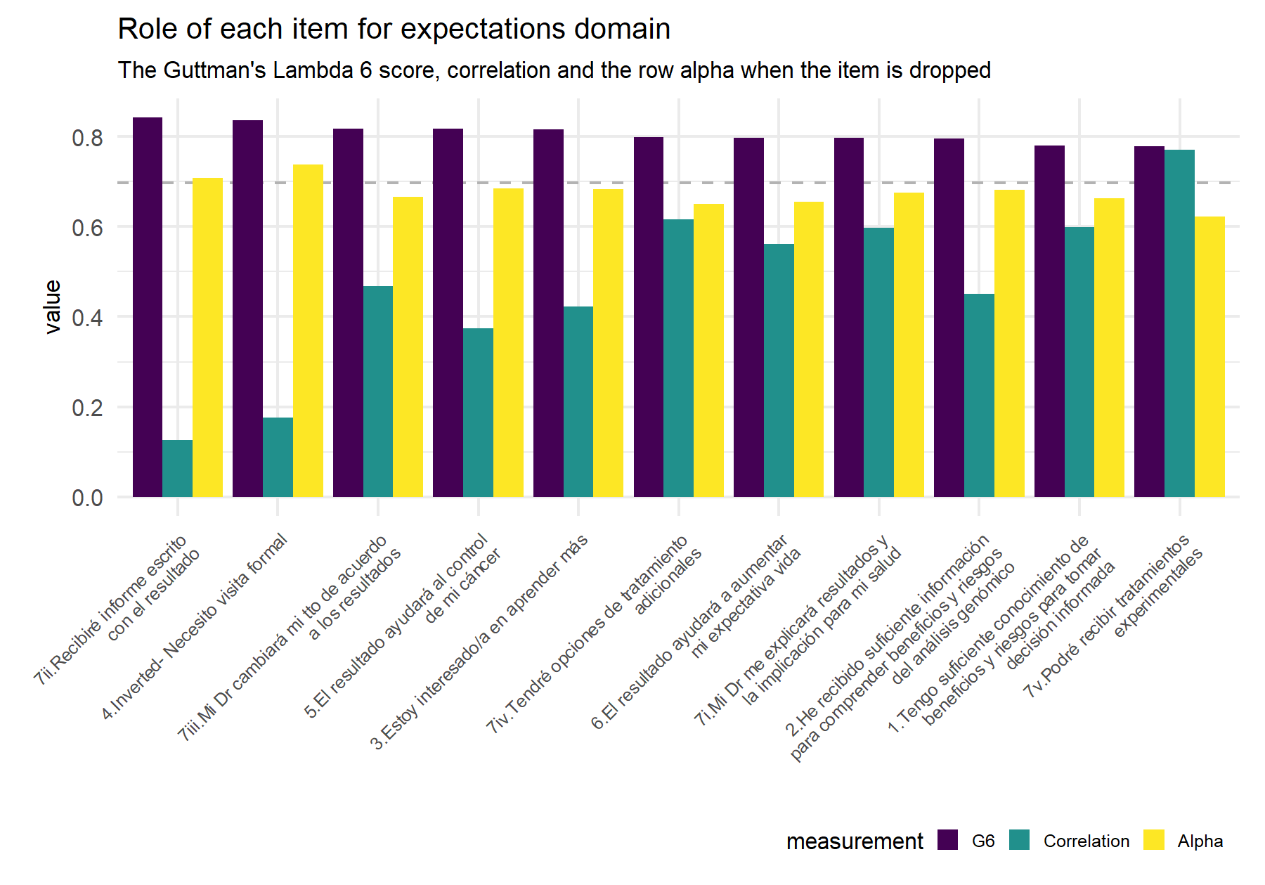
Figure 9.1: Dashed line indicates the alpha (Feldt alpha) value for the whole set of items in order to compare this value if the alpha value that results from dropping the corresponding item (yellow bar).
| Items | G6 | raw_alpha_itemDropped | r.cor |
|---|---|---|---|
| 7ii.Recibiré informe escrito con el resultado | 0.8427 | 0.7086 | 0.1265 |
| 4.Inverted- Necesito visita formal | 0.8359 | 0.7378 | 0.1765 |
| 7iii.Mi Dr cambiará mi tto de acuerdo a los resultados | 0.8180 | 0.6667 | 0.4682 |
| 5.El resultado ayudará al control de mi cáncer | 0.8169 | 0.6851 | 0.3748 |
| 3.Estoy interesado/a en aprender más | 0.8160 | 0.6830 | 0.4220 |
| 7iv.Tendré opciones de tratamiento adicionales | 0.7987 | 0.6500 | 0.6164 |
| 6.El resultado ayudará a aumentar mi expectativa vida | 0.7978 | 0.6552 | 0.5610 |
| 7i.Mi Dr me explicará resultados y la implicación para mi salud | 0.7973 | 0.6752 | 0.5979 |
| 2.He recibido suficiente información para comprender beneficios y riesgos del análisis genómico | 0.7950 | 0.6811 | 0.4513 |
| 1.Tengo suficiente conocimiento de beneficios y riesgos para tomar decisión informada | 0.7805 | 0.6629 | 0.5991 |
| 7v.Podré recibir tratamientos experimentales | 0.7778 | 0.6231 | 0.7712 |
Describing and summarizing the results, Q4 inv and Q7.ii show the worst scores. Besides, Q7.iii, Q3, Q5, and Q2 have lower correlation scores with higher values for alpha when the item is dropped (there is a small gap between these values and the hole alpha value).
Results are not equal between cohorts (VHIO and HOPE). There is a naturally discrepancy related with each population and study. For instance, for item 7.ii regarding the written report, in HOPE is clearly specified this when the patient is enrolled. On the other hand, similarly as what was seen in the VHIO cohort, item 4 in does not work correctly.
Then, as an exploratory analysis, item 7.iii is inverted and results evaluated.
##
##    95% confidence boundaries (Feldt)
##  lower alpha upper
## 0.27 0.5 0.69| Omega (total) |
|---|
| 0.4374 |
| Items | G6 | raw_alpha_itemDropped | r.cor |
|---|---|---|---|
| 7v.Podré recibir tratamientos experimentales | 0.6958 | 0.3782 | 0.7292 |
| 7i.Mi Dr me explicará resultados y la implicación para mi salud | 0.7109 | 0.4486 | 0.6543 |
| 1.Tengo suficiente conocimiento de beneficios y riesgos para tomar decisión informada | 0.6925 | 0.4168 | 0.6350 |
| 7iv.Tendré opciones de tratamiento adicionales | 0.7244 | 0.4177 | 0.5867 |
| 2.He recibido suficiente información para comprender beneficios y riesgos del análisis genómico | 0.7082 | 0.4281 | 0.5426 |
| 6.El resultado ayudará a aumentar mi expectativa vida | 0.7283 | 0.4410 | 0.4962 |
| 3.Estoy interesado/a en aprender más | 0.7558 | 0.4959 | 0.3326 |
| 5.El resultado ayudará al control de mi cáncer | 0.7554 | 0.4902 | 0.3051 |
| 4.Inverted- Necesito visita formal | 0.7689 | 0.5029 | 0.2532 |
| 7ii.Recibiré informe escrito con el resultado | 0.7824 | 0.5065 | 0.1562 |
| 7iii.Inverted- Mi Dr cambiará mi tto inmediatamente | 0.8180 | 0.6667 | -0.4082 |
When this item is inverted, the scores decrease. Alpha value dropped from 0.7 to 0.5 as well as for omega which falls from 0.79 to 0.44. Besides, scores for this item are conflicting with a negative correlation and increasing the total alpha when the item is dropped.
9.3.2.2 Concerns
Regarding concerns, the last 4 questions are focus on this topic. These questions are analyzed without reverting the scale (i.e., in the same direction that the patient completed it).
First, analyzing the reliability of the whole subset of items, i.e., the consistency of the concerns section several measurements are display: the Cronbach’s α, with its IC, and the omega (ω) coefficient.
##
##    95% confidence boundaries (Feldt)
##  lower alpha upper
##   0.59  0.74  0.84
##
## Information about this analysis:
##
## Dataframe: pre_test_Q_Concerns_values
## Items: all
## Observations: 48
## Positive correlations: 6 out of 6 (100%)
##
## Estimates assuming interval level:
##
## Omega (total): 0.83
## Omega (hierarchical): 0.52
## Revelle's omega (total): 0.83
## Greatest Lower Bound (GLB): NA
## Coefficient H: 1
## Coefficient alpha: 0.74
##
## (Estimates assuming ordinal level not computed, as the polychoric correlation matrix has missing values.)
##
## Note: the normal point estimate and confidence interval for omega are based on the procedure suggested by Dunn, Baguley & Brunsden (2013) using the MBESS function ci.reliability, whereas the psych package point estimate was suggested in Revelle & Zinbarg (2008). See the help ('?scaleStructure') for more information.Then, in order to inspect the role of each item, the r.cor and the Guttman’s Lambda 6 (G6) are explored.
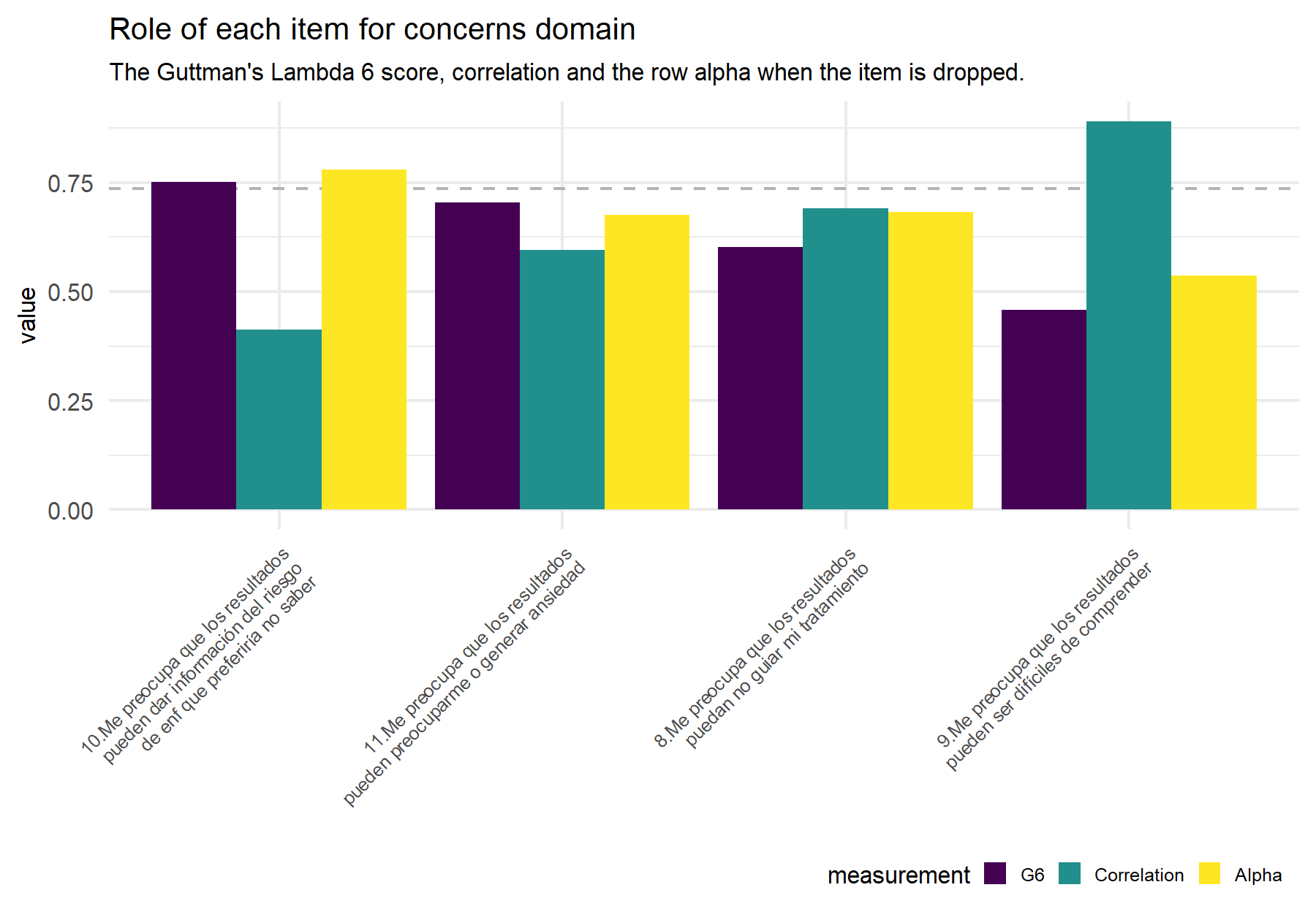
Figure 9.2: Dashed line indicates the alpha (Feldt alpha) value for the whole set of items in order to compare this value if the alpha value that results from dropping the corresponding item (yellow bar).
##                                                                                                Items
## 1 10.Me preocupa que los resultados pueden dar información del riesgo de enf que preferiría no saber
## 2                                            11.Los resultados pueden preocuparme o generar ansiedad
## 3                                    8.Me preocupa que los resultados puedan no guiar mi tratamiento
## 4                                9.Me preocupa que los resultados pueden ser difíciles de comprender
##       G6 raw_alpha_itemDropped  r.cor
## 1 0.7508                0.7789 0.4132
## 2 0.7034                0.6758 0.5949
## 3 0.6015                0.6815 0.6907
## 4 0.4575                0.5360 0.8906
Analyzing these items, concerns seem to be well captured with a Cronbach’s α of 0.74 and the omega coefficient of 0.83; showing lower values than in the VHIO cohort. Then, the evaluation of each item shows opposite score results for G6 and r.cor, and some discrepancies with the VHIO cohort. While here the lowest r.cor is observed for item 10 in the VHIO study this item showed the highest correlation. Contrary, the highest correlation here is for item 9 which was the item with the lowest correlation previously. Nevertheless, the best combination of both scores is for item 11 and 8, equal to the VHIO cohort.
9.3.3 Global conclusions about expectations domain
Similar to the approach in the VHIO cohort, some items could be identified as less relevant and other as more relevant when all these prior steps are taken together.
Therefore, for expectations, it is possible to summarize the findings as follows:
summary variability and discrimination-
The best five elements are: Q6, Q7.v, Q5, Q7.iv, and Q7.i.
The worst two: Q4 and Q7.ii.
Conflicting results: item Q2, showing a discrimination score below the threshold.
Summary G6, alpha, and correlation-
The best items: Q7.v, Q6, Q7.iv, Q7.i, and Q1. Q7.iii shows high G6 scores but low correlation.
The worst items Q4 and Q7.ii.
Best potential items:
Q6, Q7.v, Q7.iv, and Q7.i.
Potential items to be excluded:
Q4 and Q7.ii are probably the first items to be excluded according to the previous findings, and these results.
Then, there are other conflicting items, principally, because they show different results between cohorts. For instance, in this cohort Q1 has better scores than Q2, while in the VHIO cohort results were the opposite. Besides, Q7.iii exhibit here better results than in the VHIO cohort. On the contrary, Q5 did not present the highest values found in the VHIO cohort.
With regard to the concerns domain, the there is not a clear difference between them. At least, item 11 seem to be relevant. The second item to be chosen can be identify when the rest of the analysis were completed.
9.4 Attitudes domain
This domain includes 11 items. Out of these, 8 are questions with a Likert scale and 3 are items to select one or more options. These last 3 items are oriented to the patient´s motivation for performing the genomic testing. In the HOPE questionnaire, item 9 was included in the platform in a wrong way; instead of allowing one option it was built to select more than one. Thus, as a result, this item could not be used in this analysis.
For attitudes items, number 5 should be interpreted in an opposite way:
- item 5. “El análisis genómico parece ser una prueba imprecisa.”. Independently that this questionnaire is focused on patients point of view, clearly, genomic testing are precise assays. Later, for the analysis this question will be inverted.
9.4.1 Visualizing items and responses
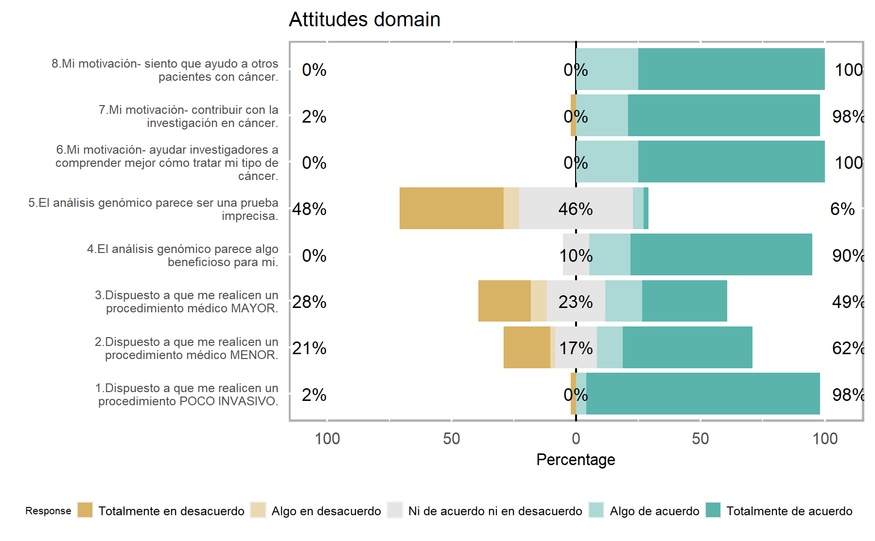
In this setting, when again similar trends are detected, there are differences that can be associated with each study design. For instance, in HOPE more are keen on to have a new blood sample, and with regards to motivation items virtually all agree completely.
Secondly, the difficulty and discrimination capacity is evaluated for each of these items.
## Warning: Estimated discrimination is lower than 0.## Scale for fill is already present.
## Adding another scale for fill, which will replace the existing scale.
## Scale for colour is already present.
## Adding another scale for colour, which will replace the existing scale.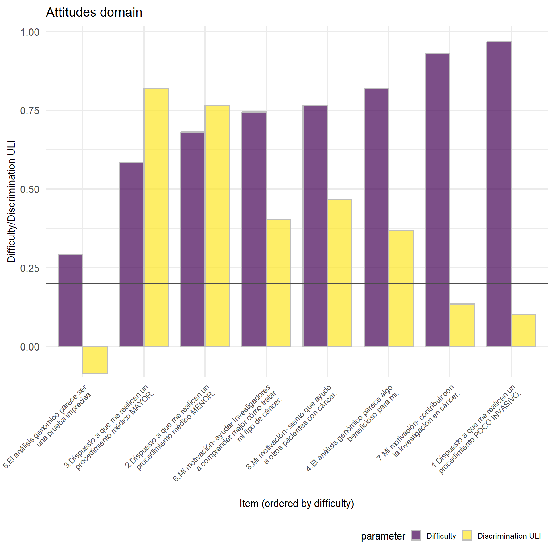
Similarly to what was seen in the VHIO cohort, item Q5 has a negative discrimination score; then, items Q3 and Q2 are those with the highest discrimination. In this setting, item Q1 showed a lower value than in VHIO, probably related to the study designed and the set of patients enrolled. Then, item 4 has a moderate discrimination in both studies.
Partial conclusion:
Variability- Highest variability: Q5, Q3, and Q2.
Lowest variability: items Q8, Q6, Q7, and Q1.
Discrimination- Highest discrimination: items 3, and 2.
Lowest discrimination: items Q5, Q7, and Q1.
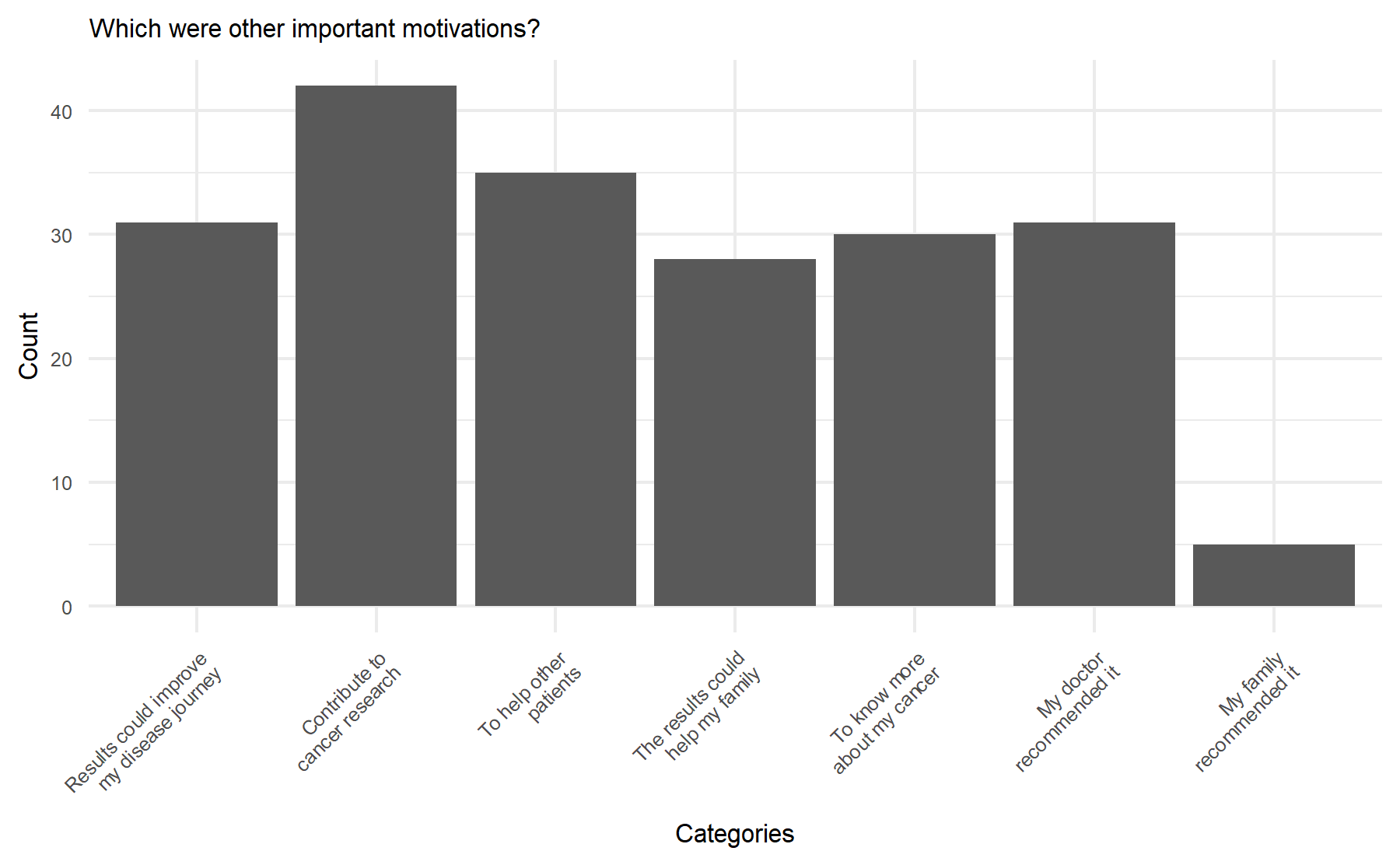
Additionally, there are three last questions focused on motivations with multiple choice options. Two asking about the mains motivations, and one to determine the less relevant motivation. These results are depict graphically below.
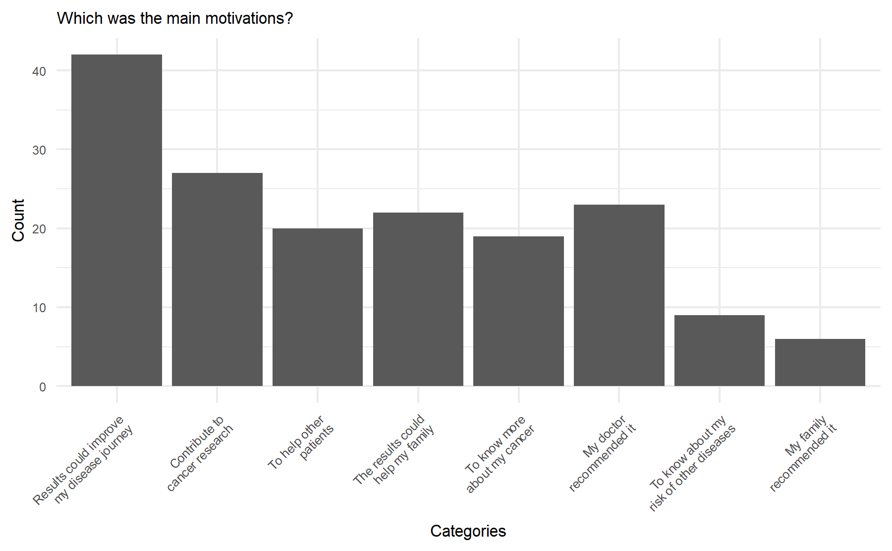
 According to these results, the key motivation to pursue genomic testing were to improve the journey or evolution of their disease followed by to contribute to cancer research and to help other patients.
Then, the less relevant topic was:
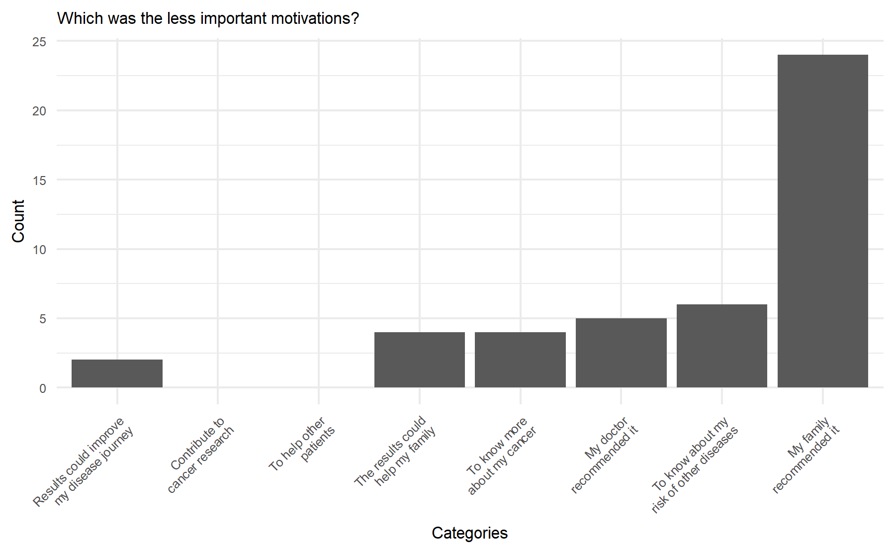 In this setting the less significant motivation was their family recommended it.
9.4.2 Evaluating the reliability of questions (Cronbach’s α and Omega)
The Cronbach’s α and the Guttman’s lambda_6 (G6) are calculated for the attitude domain.
##
##    95% confidence boundaries (Feldt)
##  lower alpha upper
## 0.62 0.74 0.84| Omega (total) |
|---|
| 0.9032 |
| Omega (hierarchical) |
|---|
| 0.4116 |
Item 5 continue showing conflict results. Alpha was 0.74 and omega 0.9.
Then, in order to inspect the role of each item, the r.cor and the Guttman’s Lambda 6 (G6) are explored.
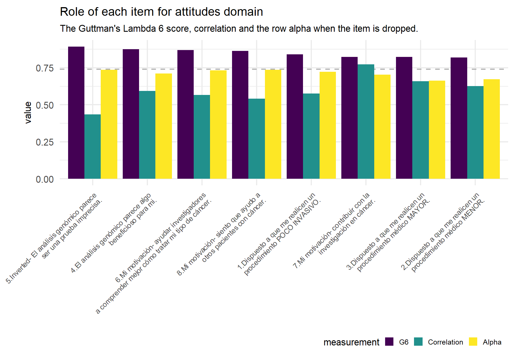
Figure 9.3: Dashed line indicates the alpha (Feldt alpha) value for the whole set of items in order to compare this value if the alpha value that results from dropping the corresponding item (yellow bar).
| Items | G6 | raw_alpha_itemDropped | r.cor |
|---|---|---|---|
| 5.Inverted- El análisis genómico parece ser una prueba imprecisa. | 0.8930 | 0.7370 | 0.4352 |
| 4.El análisis genómico parece algo beneficioso para mi. | 0.8752 | 0.7119 | 0.5928 |
| 6.Mi motivación- ayudar investigadores a comprender mejor cómo tratar mi tipo de cáncer. | 0.8699 | 0.7318 | 0.5661 |
| 8.Mi motivación- siento que ayudo a otros pacientes con cáncer. | 0.8639 | 0.7367 | 0.5412 |
| 1.Dispuesto a que me realicen un procedimiento POCO INVASIVO. | 0.8413 | 0.7229 | 0.5767 |
| 7.Mi motivación- contribuir con la investigación en cáncer. | 0.8231 | 0.7041 | 0.7734 |
| 3.Dispuesto a que me realicen un procedimiento médico MAYOR. | 0.8231 | 0.6636 | 0.6589 |
| 2.Dispuesto a que me realicen un procedimiento médico MENOR. | 0.8195 | 0.6734 | 0.6268 |
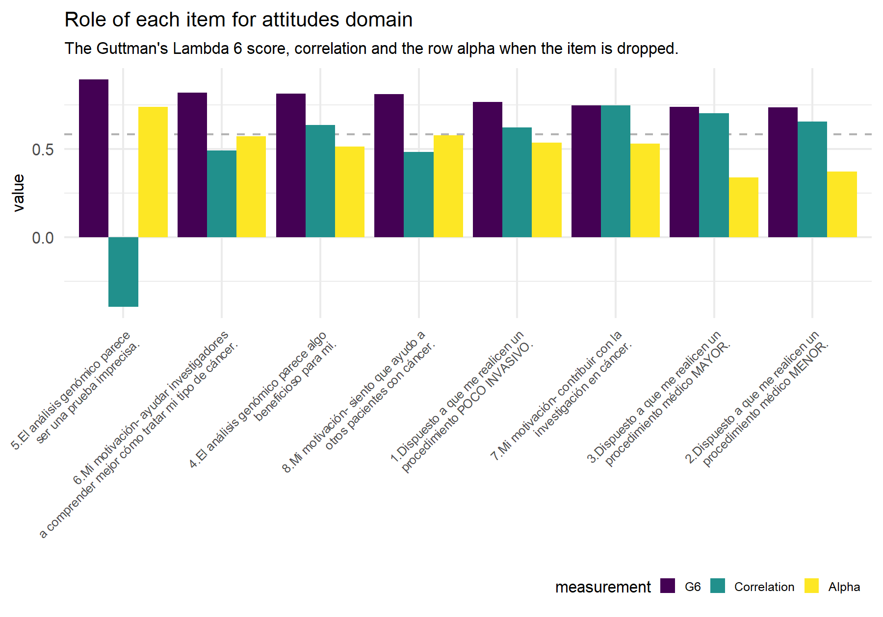
Figure 9.4: Dashed line indicates the alpha (Feldt alpha) value for the whole set of items in order to compare this value if the alpha value that results from dropping the corresponding item (yellow bar).
| Items | G6 | raw_alpha_itemDropped | r.cor |
|---|---|---|---|
| 5.El análisis genómico parece ser una prueba imprecisa. | 0.8930 | 0.7370 | -0.3946 |
| 6.Mi motivación- ayudar investigadores a comprender mejor cómo tratar mi tipo de cáncer. | 0.8192 | 0.5725 | 0.4903 |
| 4.El análisis genómico parece algo beneficioso para mi. | 0.8131 | 0.5125 | 0.6365 |
| 8.Mi motivación- siento que ayudo a otros pacientes con cáncer. | 0.8098 | 0.5782 | 0.4825 |
| 1.Dispuesto a que me realicen un procedimiento POCO INVASIVO. | 0.7665 | 0.5352 | 0.6200 |
| 7.Mi motivación- contribuir con la investigación en cáncer. | 0.7458 | 0.5292 | 0.7454 |
| 3.Dispuesto a que me realicen un procedimiento médico MAYOR. | 0.7384 | 0.3380 | 0.7025 |
| 2.Dispuesto a que me realicen un procedimiento médico MENOR. | 0.7365 | 0.3711 | 0.6547 |
The capture of the attitude domain is adequate with a Cronbach’s α of 0.74 and the omega coefficient of 0.90, being these results close to previous ones. Similarly to the VHIO study the three items with the highest correlation are Q3, Q2 and Q7. Q2 and Q3 showed the lowest G6 with the best values of correlation and alpha when the item is dropped. For Q4 the correlation and the alpha when the item is dropped is not as high but the G6 is the second largest. Then item 5 inverted works better than in VHIO but it shows the lower correlation; when it is not inverted, the correlation is negative.
9.4.3 Global conclusions about attitude domain
The highest variability and discrimination were seen for items Q3, Q2, and Q5. While the lowest were found for Q8, Q7, and Q1. Item Q5 showed the highest variability and the worst discrimination capacity. Considering the G6, alpha and the correlation score, while the best ones are Q3, and Q2, followed by Q7 and Q4.
Similar to what was proposed before, the possible approach is to exclude all the motivation items, Q6, Q7, and Q8; but including Q9 in which the patient select its main motivation. Then, to have the final set of 5 items, an additional one from Q1-Q5 should be excluded. In this line, item 5 showed the lower discrimination score and the worst alpha and correlation. However, Q1 probably it is no adding any relevant information.
Therefore, the list includes: Q2, Q3, and Q4, plus Q9. And potentially, Q5.