Chapter 8 Post-test Questionnaire- Factor analysis
At this stage, the main objective is to perform an exploratory factor analysis focusing on previous results. The pre-genomic test data analysis allows to identify items that are less relevant and which are the most informative ones, questions with adequate behavior, and how they group. The descriptive analysis of the post-genomic test questionnaire highlighted several common points with the pre-genomic test information, detecting a few conflicting items and the utility of those selected in the previous step. Now, having identified from the pre-genomic test exploratory factor analysis a few key approaches, the aim is to replicate only these factor analyses including the set of items that had been chosen to explore and define how they group in this setting.
8.1 Expectations and concerns domain
One approach is considered including the final set of expectations and concerns items. In this regard, expectations questions include Q2, Q5, Q5, Q7.i, Q7.iv, Q7.v, and all the concerns items. This approach had the best performance in both cohorts, however the matching between VHIO and HOPE was not complete.
8.1.1 Excluding items Q1, Q4, Q7_ii, Q7_iii and Q3.
According to what was defined previously, Q1, Q4, Q7.ii were conflicting, overlapped (Q1 with Q2), with no relevant information, and study dependent (Q7.ii). Then, Q7_iii and Q3 are collecting interesting data but probably they are not related with the other questions in a particular domain; thus, while these items will be included in the questionnaire, they could be excluded from the factor analysis.
The Barlett’s sphericity test is performed.
Thus, the p-value = 0 and the H0 is rejected confirming the utility of applying a factor analysis to this dataset.
Considering the fact that the Bartlett’s test usually rejects the H0 since the scenario of the null hypothesis is too extreme, the KMO analysis is studied to determine how well the data fit the factor analysis and how useful each item is.
## Kaiser-Meyer-Olkin factor adequacy
## Call: KMO(r = post_test_Q_ExpConcern_facAn_4_corr)
## Overall MSA =  0.54
## MSA for each item =
##    q2    q5    q6  q7_i q7_iv  q7_v    q8    q9   q10   q11
##  0.41  0.74  0.56  0.48  0.50  0.86  0.62  0.36  0.68  0.44
According to these results, there four items below 0.5 Q2, Q7.i, Q9, Q11; plus two more below 0.6.
To explore the number of factors PCA is applied. Thus, the table with the PCA results is shown below:
| PC1 | PC2 | PC3 | PC4 | PC5 | PC6 | PC7 | PC8 | PC9 | PC10 | |
|---|---|---|---|---|---|---|---|---|---|---|
| Standard deviation | 1.8484 | 1.6684 | 1.1822 | 0.9659 | 0.7358 | 0.6070 | 0.5164 | 0.4004 | 0.2971 | 0.2102 |
| Proportion of Variance | 0.3417 | 0.2784 | 0.1398 | 0.0933 | 0.0541 | 0.0368 | 0.0267 | 0.0160 | 0.0088 | 0.0044 |
| Cumulative Proportion | 0.3417 | 0.6200 | 0.7598 | 0.8531 | 0.9072 | 0.9441 | 0.9707 | 0.9868 | 0.9956 | 1.0000 |
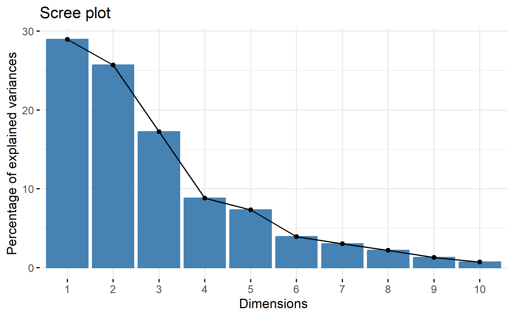
Then, the scree plot for this PCA analysis is displayed.
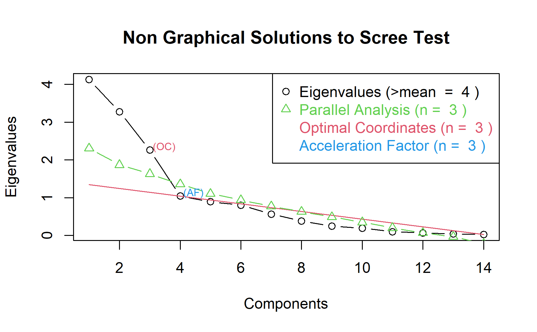
 According to these results, 2-3 factors could be the best number. While the cumulative proportion with 2 components is 62%, and with three 76%; beside, an elbow can be identified on the third component.
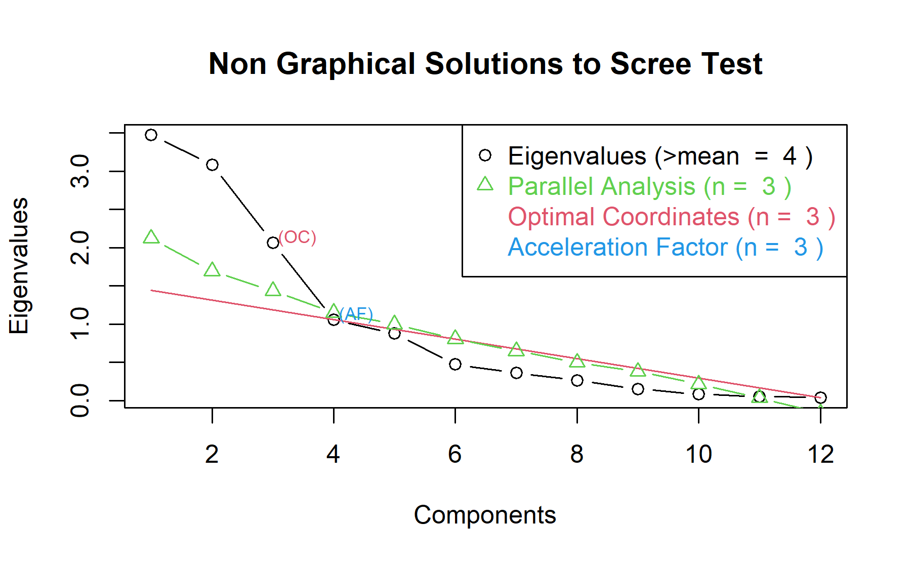
Then, another approach is implemented. With this strategy several analysis are combined and depict in the same figure. The tools implemented are: the Kaiser rule (which drops the components with eigenvalues < 1), the parallel analysis, and the usual scree test (plotuScree), the acceleration factor (which indicates where the elbow of the scree plot appears).
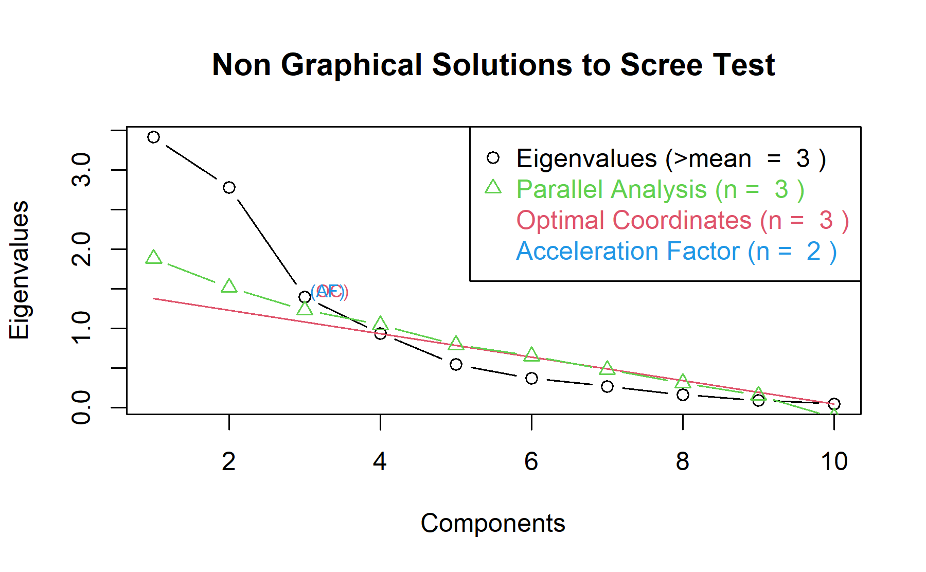 Therefore, considering the current analysis three factors seem to be the best choice, however, in the pre-genomic test two factors were identified. Therefore, both approaches will be considered.
Running the factor analysis with 10 items and 3 factors, first the communalities are explored:
## Warning in cor.smooth(mat): Matrix was not positive definite, smoothing was
## done
## In factor.stats, I could not find the RMSEA upper bound . Sorry about that## post_exp_preoc_q2 post_exp_preoc_q5 post_exp_preoc_q6
## 0.6681 0.8150 0.9950
## post_exp_preoc_q7_i post_exp_preoc_q7_iv post_exp_preoc_q7_v
## 0.9950 0.7618 0.6935
## post_exp_preoc_q8 post_exp_preoc_q9 post_exp_preoc_q10
## 0.6211 0.9950 0.6395
## post_exp_preoc_q11
## 0.7771Considering the values of the communalities, all are above 0.6.
Then, the whole output is displayed.
## Factor Analysis using method = ml
## Call: fa(r = post_test_Q_ExpConcern_facAn_4, nfactors = 3, rotate = "oblimin",
## fm = "ml", cor = "poly")
## Standardized loadings (pattern matrix) based upon correlation matrix
## ML2 ML1 ML3 h2 u2 com
## post_exp_preoc_q2 0.84 0.67 0.3319 1.3
## post_exp_preoc_q5 0.90 0.81 0.1850 1.1
## post_exp_preoc_q6 0.99 1.00 0.0049 1.0
## post_exp_preoc_q7_i 0.90 1.00 0.0049 1.2
## post_exp_preoc_q7_iv 0.59 0.53 0.76 0.2383 2.1
## post_exp_preoc_q7_v 0.84 0.69 0.3065 1.0
## post_exp_preoc_q8 0.64 0.62 0.3789 1.5
## post_exp_preoc_q9 0.99 1.00 0.0049 1.0
## post_exp_preoc_q10 0.65 0.64 0.3605 1.5
## post_exp_preoc_q11 0.73 0.78 0.2230 1.6
##
## ML2 ML1 ML3
## SS loadings 3.07 2.75 2.15
## Proportion Var 0.31 0.27 0.21
## Cumulative Var 0.31 0.58 0.80
## Proportion Explained 0.39 0.35 0.27
## Cumulative Proportion 0.39 0.73 1.00
##
## With factor correlations of
## ML2 ML1 ML3
## ML2 1.00 0.22 0.22
## ML1 0.22 1.00 -0.18
## ML3 0.22 -0.18 1.00
##
## Mean item complexity = 1.3
## Test of the hypothesis that 3 factors are sufficient.
##
## df null model = 45 with the objective function = 52.27 with Chi Square = 879.9
## df of the model are 18 and the objective function was 42.98
##
## The root mean square of the residuals (RMSR) is 0.1
## The df corrected root mean square of the residuals is 0.15
##
## The harmonic n.obs is 22 with the empirical chi square 18.33 with prob < 0.43
## The total n.obs was 22 with Likelihood Chi Square = 637.6 with prob < 9.7e-124
##
## Tucker Lewis Index of factoring reliability = -1.121
## RMSEA index = 1.25 and the 90 % confidence intervals are 1.196 NA
## BIC = 581.9
## Fit based upon off diagonal values = 0.96
## Measures of factor score adequacy
## ML2 ML1 ML3
## Correlation of (regression) scores with factors 1.00 1.00 1.00
## Multiple R square of scores with factors 1.00 0.99 0.99
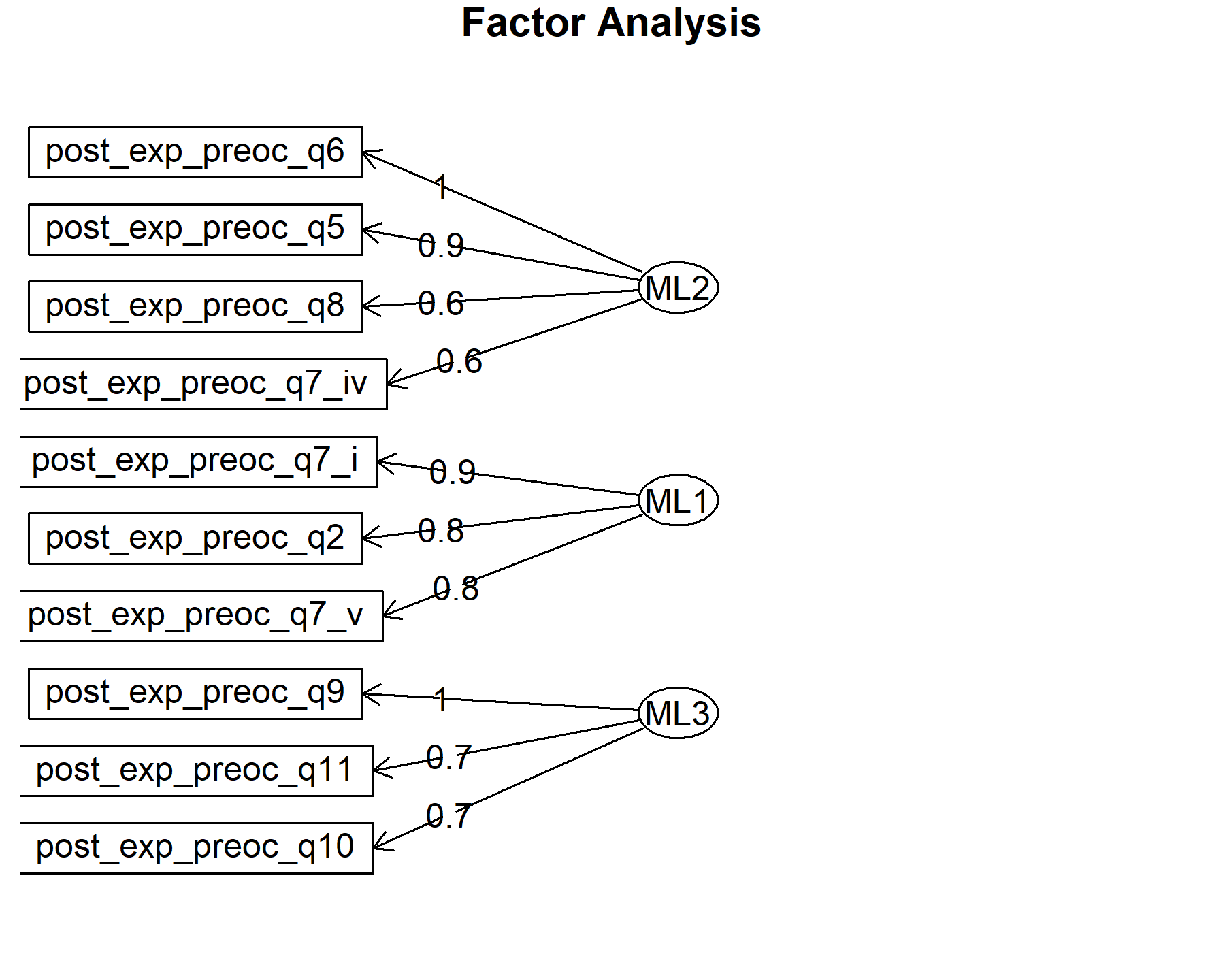
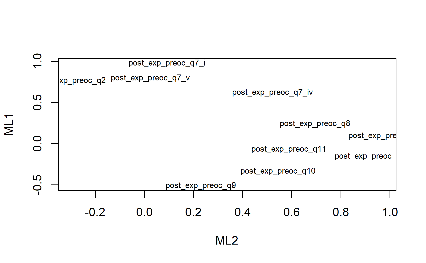
## Minimum correlation of possible factor scores 0.99 0.99 0.99There are 3 factors: * Q5, Q6, Q7_iv, Q8. * Q2, Q7.i, Q7.v, and Q7.iv * Q9, Q10, Q11. Item Q7.iv was also found linked with two factor in pre-genomic test analysis in the VHIO cohort. Nevertheless, the main different is how expectations items split into two factors including Q8 in one of these factors.
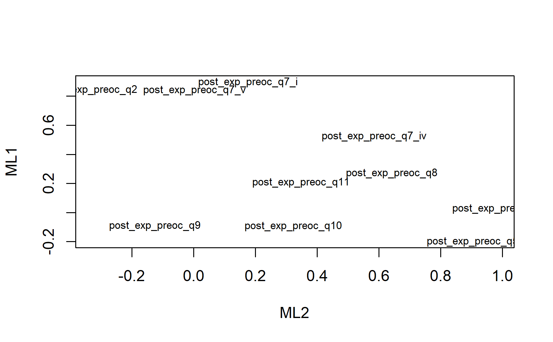
Finally, plots show the relationship between the items and the factors.
Then, the factor analysis is performed with 2 factors. The communalities are explored:
## Warning in cor.smooth(mat): Matrix was not positive definite, smoothing was
## done
## In factor.stats, I could not find the RMSEA upper bound . Sorry about that## post_exp_preoc_q2 post_exp_preoc_q5 post_exp_preoc_q6
## 0.5995 0.8215 0.9899
## post_exp_preoc_q7_i post_exp_preoc_q7_iv post_exp_preoc_q7_v
## 0.9950 0.7631 0.6397
## post_exp_preoc_q8 post_exp_preoc_q9 post_exp_preoc_q10
## 0.5974 0.2774 0.3495
## post_exp_preoc_q11
## 0.3389Considering the values of the communalities, concerns items show lower communalities.
Then, the whole output is displayed.
## Factor Analysis using method = ml
## Call: fa(r = post_test_Q_ExpConcern_facAn_4, nfactors = 2, rotate = "oblimin",
## fm = "ml", cor = "poly")
## Standardized loadings (pattern matrix) based upon correlation matrix
## ML2 ML1 h2 u2 com
## post_exp_preoc_q2 0.76 0.60 0.4009 1.3
## post_exp_preoc_q5 0.92 0.82 0.1785 1.1
## post_exp_preoc_q6 0.97 0.99 0.0101 1.0
## post_exp_preoc_q7_i 0.98 1.00 0.0049 1.0
## post_exp_preoc_q7_iv 0.52 0.62 0.76 0.2368 1.9
## post_exp_preoc_q7_v 0.80 0.64 0.3600 1.0
## post_exp_preoc_q8 0.70 0.60 0.4022 1.2
## post_exp_preoc_q9 -0.51 0.28 0.7237 1.4
## post_exp_preoc_q10 0.55 0.35 0.6495 1.7
## post_exp_preoc_q11 0.59 0.34 0.6612 1.0
##
## ML2 ML1
## SS loadings 3.34 3.03
## Proportion Var 0.33 0.30
## Cumulative Var 0.33 0.64
## Proportion Explained 0.52 0.48
## Cumulative Proportion 0.52 1.00
##
## With factor correlations of
## ML2 ML1
## ML2 1.00 0.16
## ML1 0.16 1.00
##
## Mean item complexity = 1.3
## Test of the hypothesis that 2 factors are sufficient.
##
## df null model = 45 with the objective function = 52.27 with Chi Square = 879.9
## df of the model are 26 and the objective function was 45.06
##
## The root mean square of the residuals (RMSR) is 0.16
## The df corrected root mean square of the residuals is 0.21
##
## The harmonic n.obs is 22 with the empirical chi square 51.08 with prob < 0.0023
## The total n.obs was 22 with Likelihood Chi Square = 698.5 with prob < 1.5e-130
##
## Tucker Lewis Index of factoring reliability = -0.521
## RMSEA index = 1.083 and the 90 % confidence intervals are 1.04 NA
## BIC = 618.1
## Fit based upon off diagonal values = 0.87
## Measures of factor score adequacy
## ML2 ML1
## Correlation of (regression) scores with factors 1.00 1.00
## Multiple R square of scores with factors 0.99 0.99
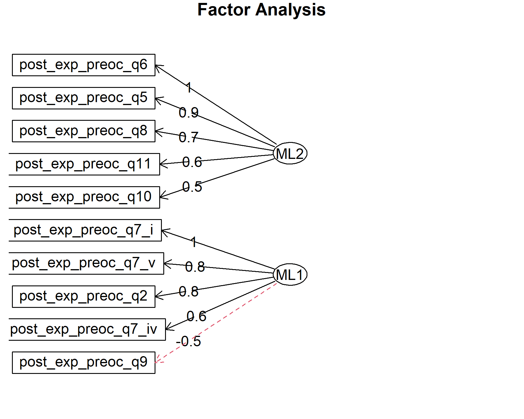
## Minimum correlation of possible factor scores 0.98 0.99There are 2 factors: * Q5, Q6, Q7_iv, Q8, Q10, Q11 * Q2, Q7.i, Q7.v, Q7.iv, and -Q9. The items are split in a completely different pattern that what was seen in the pre-genomic test questionnaire.
Finally, plots show the relationship between the items and the factors.
8.2 Both domains, the expectations and concerns domain plus the attitudes domain
Now, two other approaches combining expectations and attitudes will be tested, the first one including only the more relevant attitudes items (Q2 and Q3), and the other one considering the four candidates selected from the attitude domain. In both, the same list of previously chosen expectations and concerns items will be used.
8.2.1 Expectations plus Q2 and Q3 from attitudes.
The Barlett’s sphericity test is performed.
Thus, the p-value = 0 and the H0 is rejected confirming the utility of applying a factor analysis to this dataset.
Considering the fact that the Bartlett’s test usually rejects the H0 since the scenario of the null hypothesis is too extreme, the KMO analysis is studied to determine how well the data fit the factor analysis and how useful each item is.
## Kaiser-Meyer-Olkin factor adequacy
## Call: KMO(r = post_test_Q_Exp_Attit_facAn_1_corr)
## Overall MSA =  0.53
## MSA for each item =
##           q2           q5           q6         q7_i        q7_iv         q7_v
##         0.49         0.70         0.53         0.52         0.50         0.87
##           q8           q9          q10          q11 exp_actit_q2 exp_actit_q3
##         0.52         0.35         0.56         0.41         0.54         0.52
According to these results, there are four items below 0.5: Q2, Q9, Q11. Besides, most of the items are below 0.6.
To explore the number of factors PCA is applied. Thus, the table with the PCA results is shown below:
| PC1 | PC2 | PC3 | PC4 | PC5 | PC6 | PC7 | PC8 | PC9 | PC10 | PC11 | PC12 | |
|---|---|---|---|---|---|---|---|---|---|---|---|---|
| Standard deviation | 1.8637 | 1.7565 | 1.4381 | 1.0293 | 0.9376 | 0.6879 | 0.6026 | 0.5151 | 0.3922 | 0.2899 | 0.2324 | 0.2025 |
| Proportion of Variance | 0.2894 | 0.2571 | 0.1724 | 0.0883 | 0.0733 | 0.0394 | 0.0303 | 0.0221 | 0.0128 | 0.0070 | 0.0045 | 0.0034 |
| Cumulative Proportion | 0.2894 | 0.5466 | 0.7189 | 0.8072 | 0.8805 | 0.9199 | 0.9502 | 0.9723 | 0.9851 | 0.9921 | 0.9966 | 1.0000 |
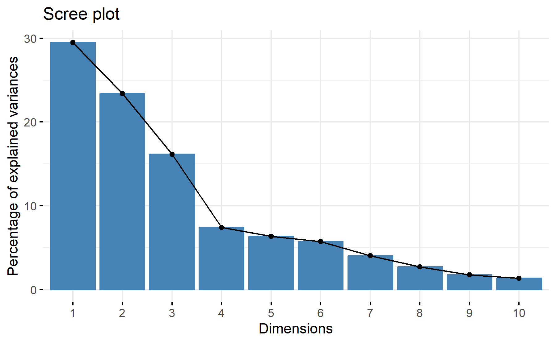
Then, the scree plot for this PCA analysis is displayed.
 According to these results, 3-4 factors could be the best number. The cumulative proportion showed that with 3 components 72% and the greater elbow is located on the four component.
Then, another approach is implemented. With this strategy several analysis are combined and depict in the same figure. The tools implemented are: the Kaiser rule (which drops the components with eigenvalues < 1), the parallel analysis, and the usual scree test (plotuScree), the acceleration factor (which indicates where the elbow of the scree plot appears).
 Therefore, considering three factors seem to be an adequate approach and is the same utilized with the pre-genomic test questionnaire.
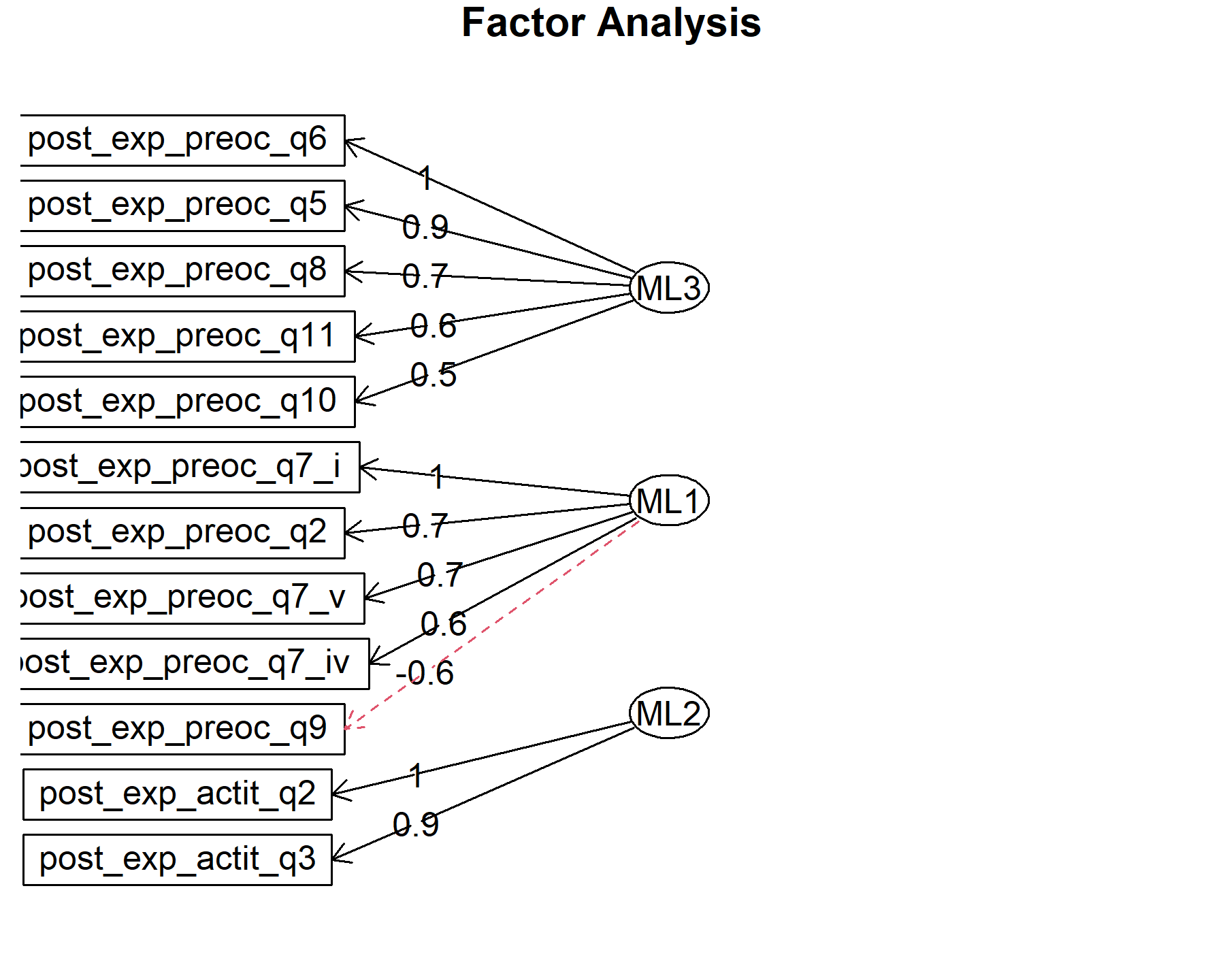
Running the factor analysis with 12 items, first the communalities are explored:
## Warning in cor.smooth(mat): Matrix was not positive definite, smoothing was
## done
## In factor.stats, I could not find the RMSEA upper bound . Sorry about that## post_exp_preoc_q2 post_exp_preoc_q5 post_exp_preoc_q6
## 0.6381 0.8623 0.9950
## post_exp_preoc_q7_i post_exp_preoc_q7_iv post_exp_preoc_q7_v
## 0.9950 0.7577 0.8003
## post_exp_preoc_q8 post_exp_preoc_q9 post_exp_preoc_q10
## 0.5998 0.4980 0.3539
## post_exp_preoc_q11 post_exp_actit_q2 post_exp_actit_q3
## 0.3789 0.9950 0.9176Considering the values of the communalities, al the items are above 0.3.
Then, the whole output is displayed.
## Factor Analysis using method =  ml
## Call: fa(r = post_test_Q_Exp_Attit_facAn_1, nfactors = 3, rotate = "oblimin",
##     fm = "ml", cor = "poly")
## Standardized loadings (pattern matrix) based upon correlation matrix
##                        ML3   ML1   ML2   h2     u2 com
## post_exp_preoc_q2           0.68       0.64 0.3617 1.6
## post_exp_preoc_q5     0.93             0.86 0.1378 1.1
## post_exp_preoc_q6     0.96             1.00 0.0050 1.1
## post_exp_preoc_q7_i         0.97       1.00 0.0049 1.0
## post_exp_preoc_q7_iv  0.52  0.64       0.76 0.2421 1.9
## post_exp_preoc_q7_v         0.67  0.45 0.80 0.1996 1.8
## post_exp_preoc_q8     0.70             0.60 0.4027 1.3
## post_exp_preoc_q9          -0.62  0.42 0.50 0.5038 2.3
## post_exp_preoc_q10    0.54             0.35 0.6466 1.6
## post_exp_preoc_q11    0.61             0.38 0.6229 1.1
## post_exp_actit_q2                 1.01 1.00 0.0049 1.0
## post_exp_actit_q3                 0.91 0.92 0.0821 1.1
##
##                        ML3  ML1  ML2
## SS loadings           3.40 2.98 2.41
## Proportion Var        0.28 0.25 0.20
## Cumulative Var        0.28 0.53 0.73
## Proportion Explained  0.39 0.34 0.27
## Cumulative Proportion 0.39 0.73 1.00
##
##  With factor correlations of
##      ML3  ML1  ML2
## ML3 1.00 0.13 0.01
## ML1 0.13 1.00 0.20
## ML2 0.01 0.20 1.00
##
## Mean item complexity =  1.4
## Test of the hypothesis that 3 factors are sufficient.
##
## df null model =  66  with the objective function =  74.97 with Chi Square =  1212
## df of  the model are 33  and the objective function was  63.84
##
## The root mean square of the residuals (RMSR) is  0.12
## The df corrected root mean square of the residuals is  0.16
##
## The harmonic n.obs is  22 with the empirical chi square  39.07  with prob <  0.22
## The total n.obs was  22  with Likelihood Chi Square =  904.4  with prob <  1.2e-168
##
## Tucker Lewis Index of factoring reliability =  -0.75
## RMSEA index =  1.095  and the 90 % confidence intervals are  1.059 NA
## BIC =  802.4
## Fit based upon off diagonal values = 0.92
## Measures of factor score adequacy
##                                                    ML3  ML1  ML2
## Correlation of (regression) scores with factors   1.00 1.00 1.00
## Multiple R square of scores with factors          0.99 0.99 1.00
## Minimum correlation of possible factor scores     0.99 0.99 0.99
There are 3 factors:
* Q5, Q6, Q7.iv, Q8, Q10, Q11
* Q2, Q7_i, Q7.iv, Q7_v, -Q9
* Q7_v, Q9, *attQ2, attQ3**.
In this setting, most of the items are split and mixed regarding the pre-genomic test exploratory factor analysis.
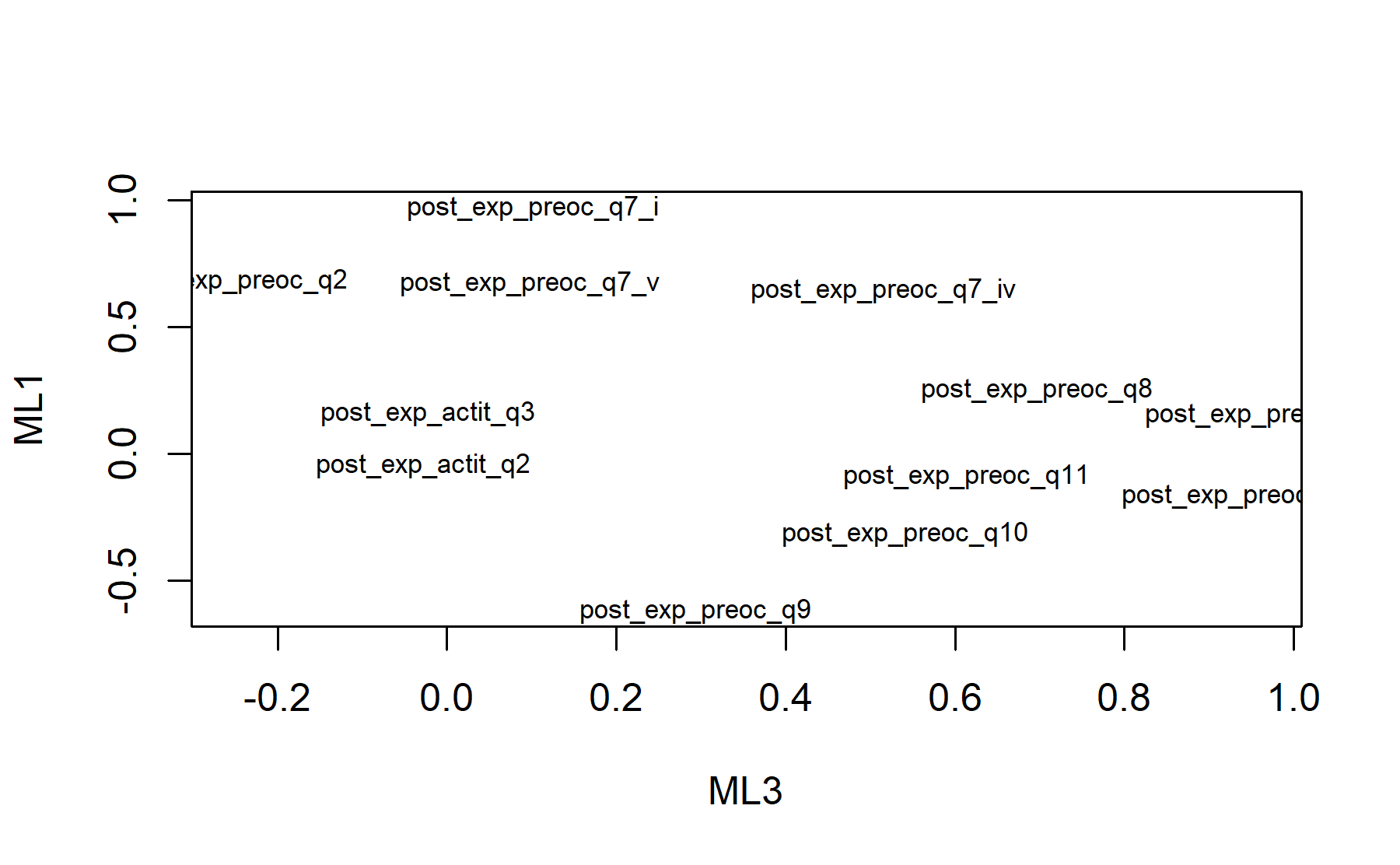
Finally, plots show the relationship between the items and the factors.
8.2.2 Expectations plus Q2, Q3, Q4, and Q5 inv from attitudes.
The Barlett’s sphericity test is performed.
Thus, the p-value = 0 and the H0 is rejected confirming the utility of applying a factor analysis to this dataset.
Considering the fact that the Bartlett’s test usually rejects the H0 since the scenario of the null hypothesis is too extreme, the KMO analysis is studied to determine how well the data fit the factor analysis and how useful each item is.
## Kaiser-Meyer-Olkin factor adequacy
## Call: KMO(r = post_test_Q_Exp_Attit_facAn_2_corr)
## Overall MSA =  0.53
## MSA for each item =
##               q2               q5               q6             q7_i
##             0.46             0.62             0.59             0.60
##            q7_iv             q7_v               q8               q9
##             0.49             0.90             0.51             0.42
##              q10              q11     exp_actit_q2     exp_actit_q3
##             0.62             0.47             0.46             0.52
##     exp_actit_q4 exp_actit_q5_Inv
##             0.50             0.42
According to these results, there is several items under the threshold of 0.5 (Q2, Q7.iv, Q9, Q11, attQ2, and attQ5 inv); moreover, most are near or below 0.6.
To explore the number of factors PCA is applied. Thus, the table with the PCA results is shown below:
| PC1 | PC2 | PC3 | PC4 | PC5 | PC6 | PC7 | PC8 | PC9 | PC10 | PC11 | PC12 | PC13 | PC14 | |
|---|---|---|---|---|---|---|---|---|---|---|---|---|---|---|
| Standard deviation | 2.0313 | 1.8101 | 1.5033 | 1.0207 | 0.9441 | 0.8948 | 0.7516 | 0.6158 | 0.4938 | 0.4366 | 0.3136 | 0.2570 | 0.1884 | 0.1591 |
| Proportion of Variance | 0.2947 | 0.2340 | 0.1614 | 0.0744 | 0.0637 | 0.0572 | 0.0403 | 0.0271 | 0.0174 | 0.0136 | 0.0070 | 0.0047 | 0.0025 | 0.0018 |
| Cumulative Proportion | 0.2947 | 0.5287 | 0.6902 | 0.7646 | 0.8283 | 0.8854 | 0.9258 | 0.9529 | 0.9703 | 0.9839 | 0.9909 | 0.9957 | 0.9982 | 1.0000 |
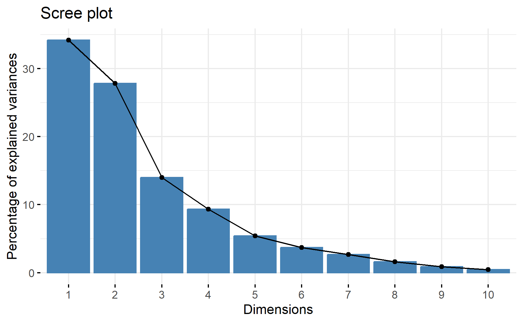
Then, the scree plot for this PCA analysis is displayed.
 According to these results, 3-4 factors could be the best number. The cumulative proportion showed that with 3 components 69% and 76% with four. While there are two elbows, the greatest one is on the four component.
Then, another approach is implemented. With this strategy several analysis are combined and depict in the same figure. The tools implemented are: the Kaiser rule (which drops the components with eigenvalues < 1), the parallel analysis, and the usual scree test (plotuScree), the acceleration factor (which indicates where the elbow of the scree plot appears).
 Therefore, considering three factors seem to be an adequate approach.
Running the factor analysis with 14 items, first the communalities are explored:
## Warning in cor.smooth(mat): Matrix was not positive definite, smoothing was
## done
## In smc, smcs < 0 were set to .0
## In smc, smcs < 0 were set to .0## In factor.stats, I could not find the RMSEA upper bound . Sorry about that## post_exp_preoc_q2 post_exp_preoc_q5
## 0.6328 0.8958
## post_exp_preoc_q6 post_exp_preoc_q7_i
## 0.9665 0.9950
## post_exp_preoc_q7_iv post_exp_preoc_q7_v
## 0.7573 0.7779
## post_exp_preoc_q8 post_exp_preoc_q9
## 0.6009 0.6087
## post_exp_preoc_q10 post_exp_preoc_q11
## 0.3811 0.4591
## post_exp_actit_q2 post_exp_actit_q3
## 0.9950 0.8837
## post_exp_actit_q4 post_exp_actit_q5_Inverted
## 0.7561 0.1915Considering the values of the communalities, while most are above 0.6, two items have lower values (attQ5 inv, and Q10).
Then, the whole output is displayed.
## Factor Analysis using method = ml
## Call: fa(r = post_test_Q_Exp_Attit_facAn_2, nfactors = 3, rotate = "oblimin",
## fm = "ml", cor = "poly")
## Standardized loadings (pattern matrix) based upon correlation matrix
## ML3 ML2 ML1 h2 u2 com
## post_exp_preoc_q2 0.61 0.63 0.3676 2.1
## post_exp_preoc_q5 0.95 0.90 0.1042 1.0
## post_exp_preoc_q6 0.97 0.97 0.0335 1.1
## post_exp_preoc_q7_i 0.94 1.00 0.0050 1.1
## post_exp_preoc_q7_iv 0.56 0.60 0.76 0.2428 2.0
## post_exp_preoc_q7_v 0.59 0.51 0.78 0.2222 2.0
## post_exp_preoc_q8 0.72 0.60 0.3991 1.1
## post_exp_preoc_q9 -0.72 0.46 0.61 0.3919 1.9
## post_exp_preoc_q10 0.51 -0.42 0.38 0.6185 1.9
## post_exp_preoc_q11 0.60 0.46 0.5416 1.7
## post_exp_actit_q2 1.02 1.00 0.0049 1.0
## post_exp_actit_q3 0.91 0.88 0.1162 1.0
## post_exp_actit_q4 0.50 0.45 0.76 0.2437 2.8
## post_exp_actit_q5_Inverted 0.42 0.19 0.8092 1.1
##
## ML3 ML2 ML1
## SS loadings 3.74 3.24 2.92
## Proportion Var 0.27 0.23 0.21
## Cumulative Var 0.27 0.50 0.71
## Proportion Explained 0.38 0.33 0.29
## Cumulative Proportion 0.38 0.71 1.00
##
## With factor correlations of
## ML3 ML2 ML1
## ML3 1.00 0.13 0.12
## ML2 0.13 1.00 0.22
## ML1 0.12 0.22 1.00
##
## Mean item complexity = 1.6
## Test of the hypothesis that 3 factors are sufficient.
##
## df null model = 91 with the objective function = 97 with Chi Square = 1407
## df of the model are 52 and the objective function was 84.36
##
## The root mean square of the residuals (RMSR) is 0.1
## The df corrected root mean square of the residuals is 0.13
##
## The harmonic n.obs is 21 with the empirical chi square 38.49 with prob < 0.92
## The total n.obs was 21 with Likelihood Chi Square = 1055 with prob < 7.8e-187
##
## Tucker Lewis Index of factoring reliability = -0.564
## RMSEA index = 0.957 and the 90 % confidence intervals are 0.931 NA
## BIC = 896.2
## Fit based upon off diagonal values = 0.94
## Measures of factor score adequacy
## ML3 ML2 ML1
## Correlation of (regression) scores with factors 0.99 1.00 1.00
## Multiple R square of scores with factors 0.98 0.99 1.00
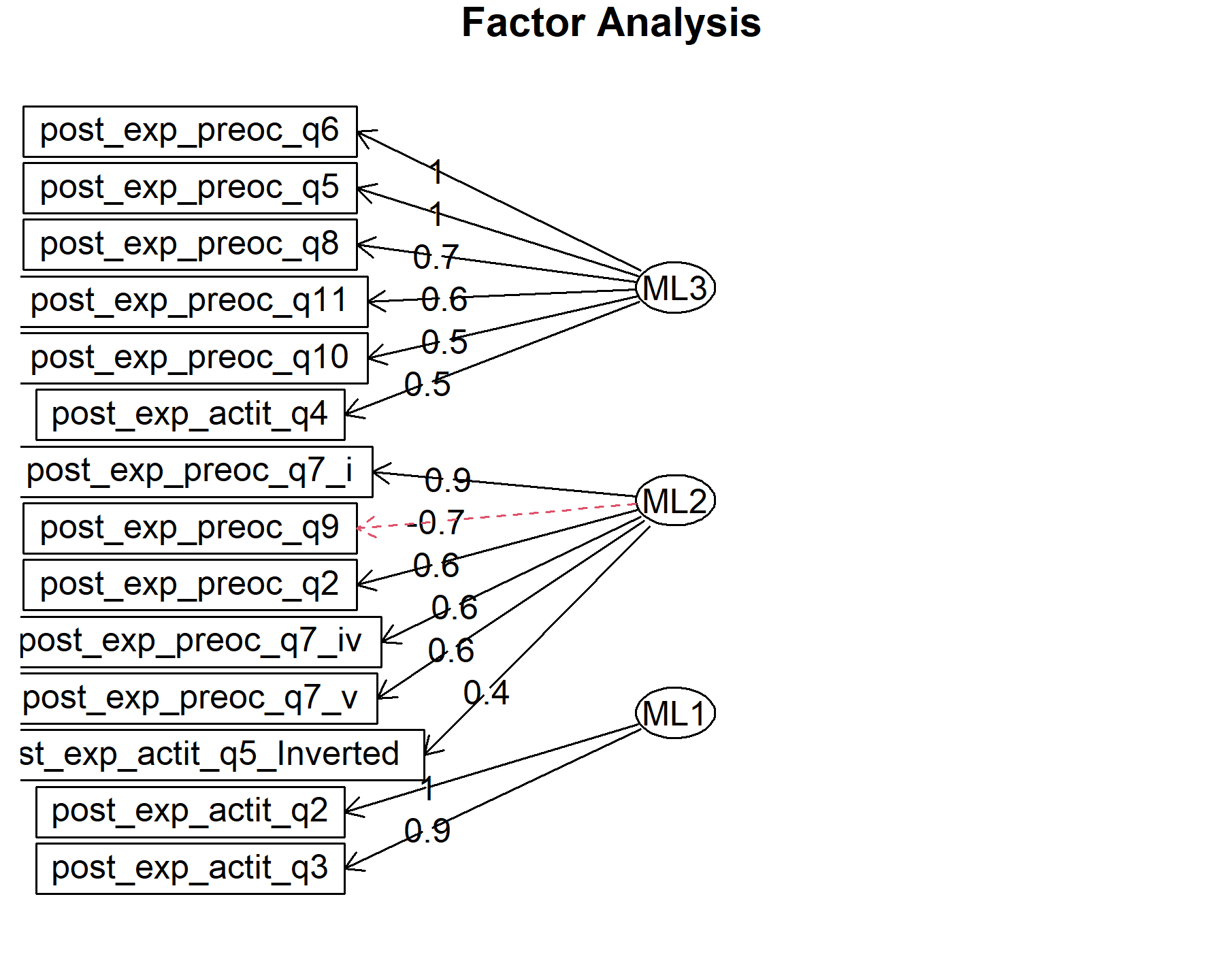
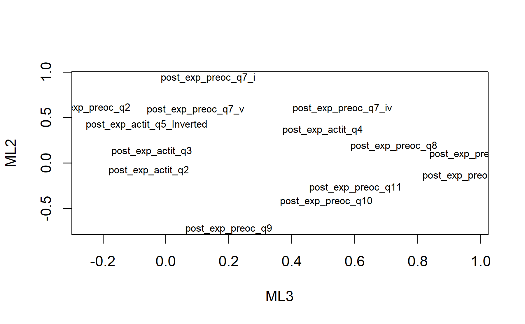
## Minimum correlation of possible factor scores 0.95 0.99 0.99There are 3 factors:
* Q5, Q6, Q7.iv, Q8, Q10, Q11, attQ4.
* Q2, Q7.i, Q7.iv, Q7.v, -Q9, -Q10, attQ5 inv.
* Q7.v, Q9, attQ2, attQ3, attQ4.
Items are mixed regarding the pre-genomic test analysis.
Finally, plots show the relationship between the items and the factors.