Chapter 10 Pre-test Questionnaire- Factor analysis
In this stage, the main idea is to perform the factor analysis with the same groups of items previously selected in order to identify is they are grouped or related in the same way.
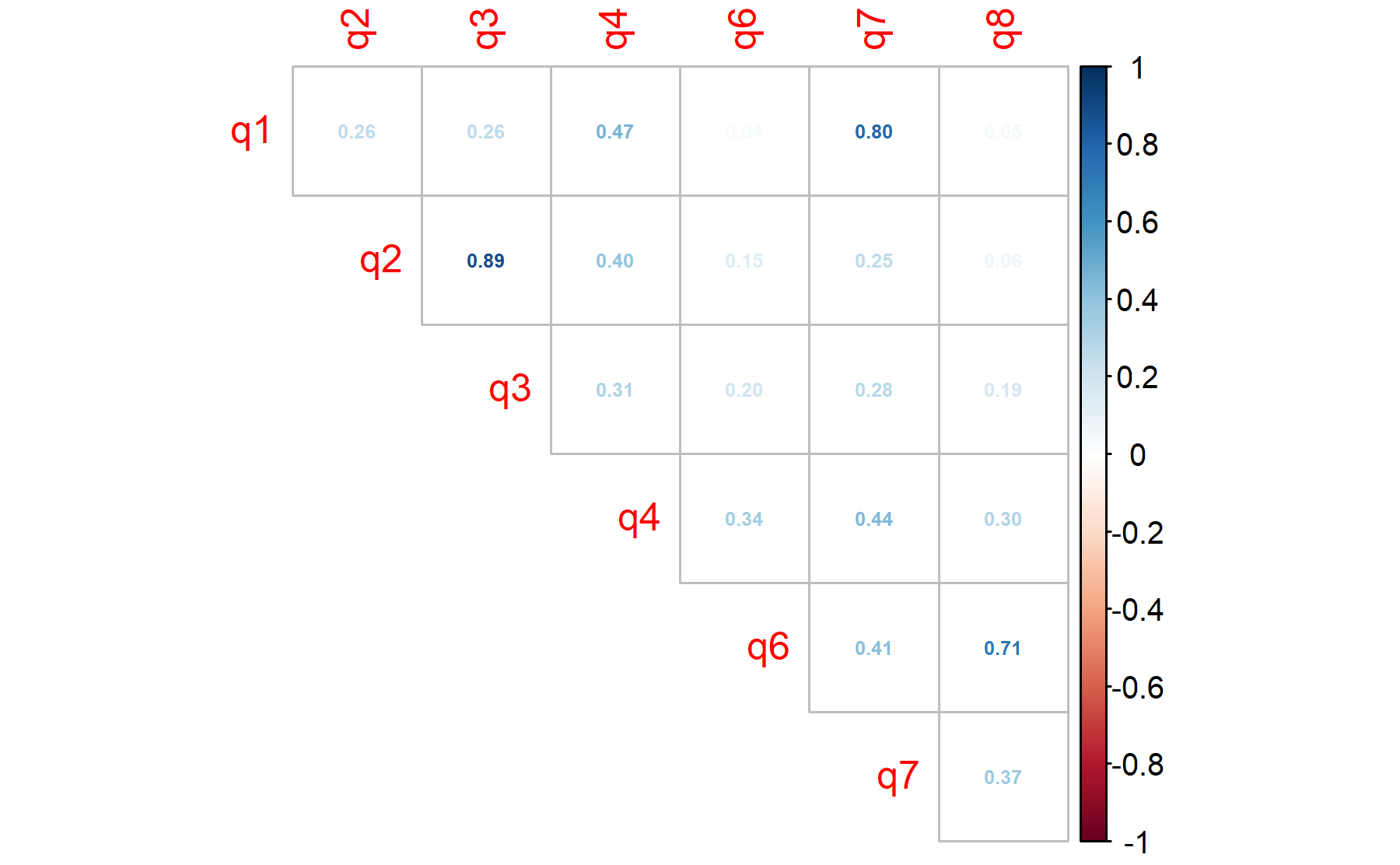
10.1 Expectations and concerns domain
10.1.1 Including all the items.
The first analysis will be done for expectations items plus concerns in order to explore the relationship between all the items. Then, the analysis will be performed for the items considered the as the chosen ones. In this first analysis, item 4 is considered inverted.
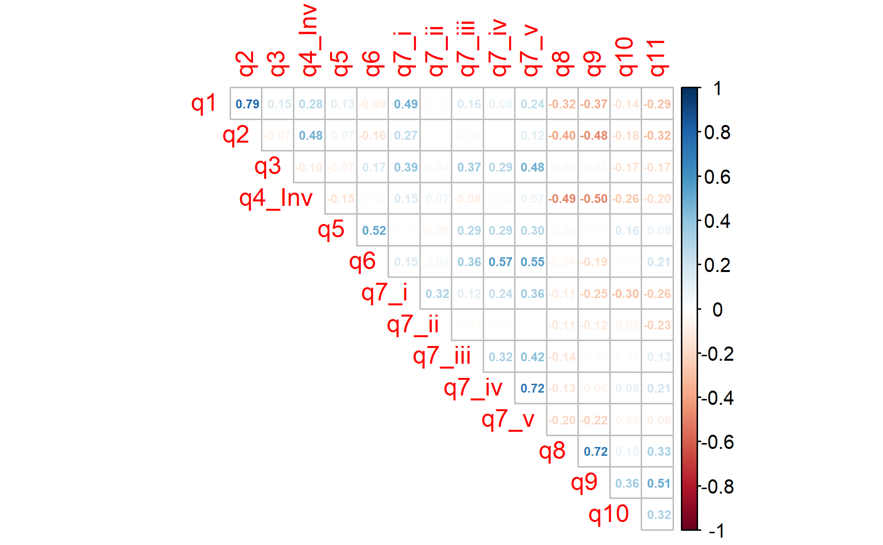
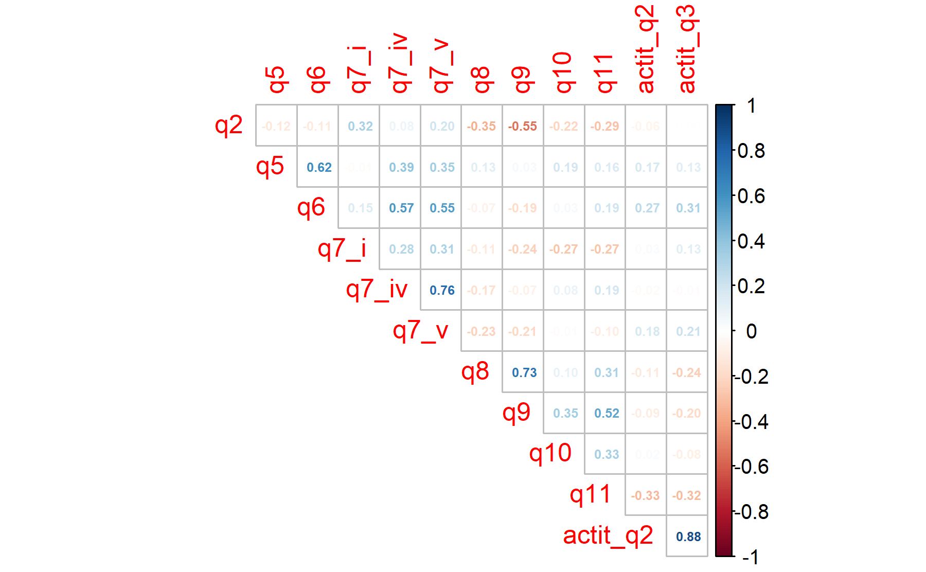
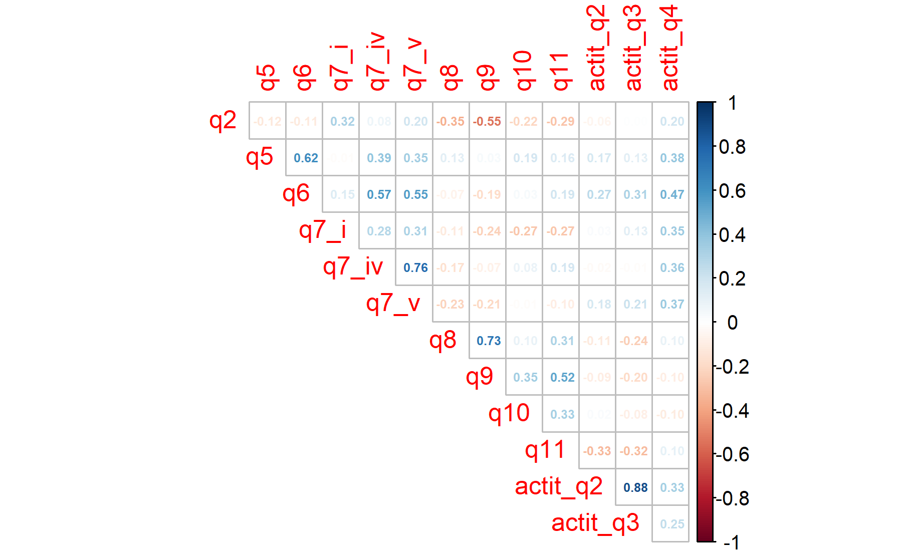
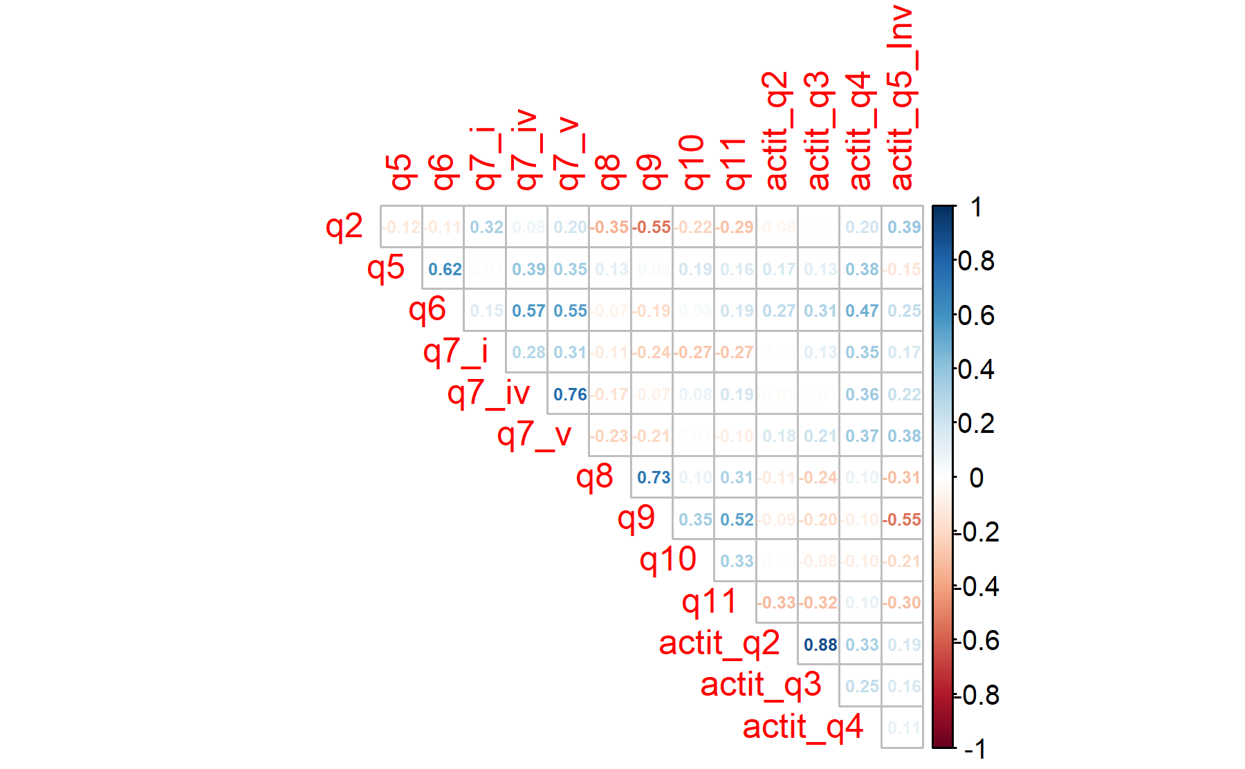
Figure 10.1: The list of the items are: 1.Tengo suficiente conocimiento de beneficios y riesgos para tomar decisión informada, 2.He recibido suficiente información para comprender beneficios y riesgos del análisis genómico, 3.Estoy interesado/a en aprender más, 4.Necesito visita formal con especialista consejo genético antes del test, 5.El resultado ayudará al control de mi cáncer, 6.El resultado ayudará a aumentar mi expectativa vida, 7i.Mi Dr me explicará resultados y la implicación para mi salud, 7ii.Recibiré informe escrito con el resultado, 7iii.Mi Dr cambiará mi tto de acuerdo a los resultados, 7iv.Tendré opciones de tratamiento adicionales, 7v.Podré recibir tratamientos experimentales, 8.Me preocupa que los resultados puedan no guiar mi tratamiento, 9.Me preocupa que los resultados pueden ser difíciles de comprender, 10.Me preocupa que los resultados pueden dar información del riesgo de enf que preferiría no saber, 11.Los resultados pueden preocuparme o generar ansiedad
As first approach the Barlett’s sphericity test is performed.
## [1] 0.0000000000000000001109Bartlett’s sphericity test provides information about whether the correlations in the data are strong enough to use a dimension-reduction technique such as principal components or common factor analysis. The test asks whether a correlation matrix is the identity matrix, a matrix containing zeros except in the diagonal which is completed by 1s. Formally speaking, it tests whether the data are a random sample from a multivariate normal population MVN(μ, Σ) where the covariance matrix Σ is a diagonal matrix (a matrix with zeros except in its diagonal). Equivalently, the variables in the population are MVN and uncorrelated. The H0 is the covariance matrix Σ is a diagonal matrix.
Thus, the p-value = 0 and the H0 is rejected confirming the utility of applying a factor analysis to this dataset.
Considering the fact that the Bartlett’s test usually rejects the H0 since the scenario of the null hypothesis is too extreme, another measurement can be studied to determine how well the data fit the factor analysis and how useful each item is. This metric is done by the KMO analysis.
Kaiser (1970) introduced a Measure of Sampling Adequacy (MSA), later modified by Kaiser and Rice (1974). The Kaiser-Meyer-Olkin (KMO) statistic, which can vary from 0 to 1, indicates the degree to which each variable in a set is predicted without error by the other variables. Kaiser (1974) suggested that KMO > .9 were marvelous, in the .80s, meritorious, in the .70s, middling, in the .60s, mediocre, in the .50s, miserable, and less than .5, unacceptable. Hair et al. (2006) suggest accepting a value > 0.5. Values between 0.5 and 0.7 are mediocre, and values between 0.7 and 0.8 are good.
Variables with individual KMO values below 0.5 could be considered for exclusion them from the analysis (note that you would need to re-compute the KMO indices as they are dependent on the whole dataset).
## Kaiser-Meyer-Olkin factor adequacy
## Call: KMO(r = pre_test_Q_ExpConcern_facAn_corr)
## Overall MSA =  0.64
## MSA for each item =
##     q1     q2     q3 q4_Inv     q5     q6   q7_i  q7_ii q7_iii  q7_iv   q7_v
##   0.61   0.62   0.66   0.73   0.52   0.56   0.65   0.39   0.70   0.72   0.75
##     q8     q9    q10    q11
##   0.62   0.63   0.69   0.63
According to these results, the Q7_ii is under the threshold of 0.5; besides, two items are below 0.6 Q5 and Q6.
To explore the number of factors that could be determined different approaches are available. First, it is possible to apply PCA and evaluate the variability explained for each component. Thus, the table with the PCA results is shown below:
| PC1 | PC2 | PC3 | PC4 | PC5 | PC6 | PC7 | PC8 | PC9 | PC10 | PC11 | PC12 | PC13 | PC14 | PC15 | |
|---|---|---|---|---|---|---|---|---|---|---|---|---|---|---|---|
| Standard deviation | 1.9413 | 1.7171 | 1.2493 | 1.1254 | 1.0245 | 0.9461 | 0.9407 | 0.8401 | 0.6702 | 0.6491 | 0.5646 | 0.5280 | 0.4462 | 0.3801 | 0.3298 |
| Proportion of Variance | 0.2512 | 0.1966 | 0.1041 | 0.0844 | 0.0700 | 0.0597 | 0.0590 | 0.0471 | 0.0300 | 0.0281 | 0.0213 | 0.0186 | 0.0133 | 0.0096 | 0.0073 |
| Cumulative Proportion | 0.2512 | 0.4478 | 0.5519 | 0.6363 | 0.7063 | 0.7659 | 0.8249 | 0.8720 | 0.9019 | 0.9300 | 0.9513 | 0.9698 | 0.9831 | 0.9928 | 1.0000 |
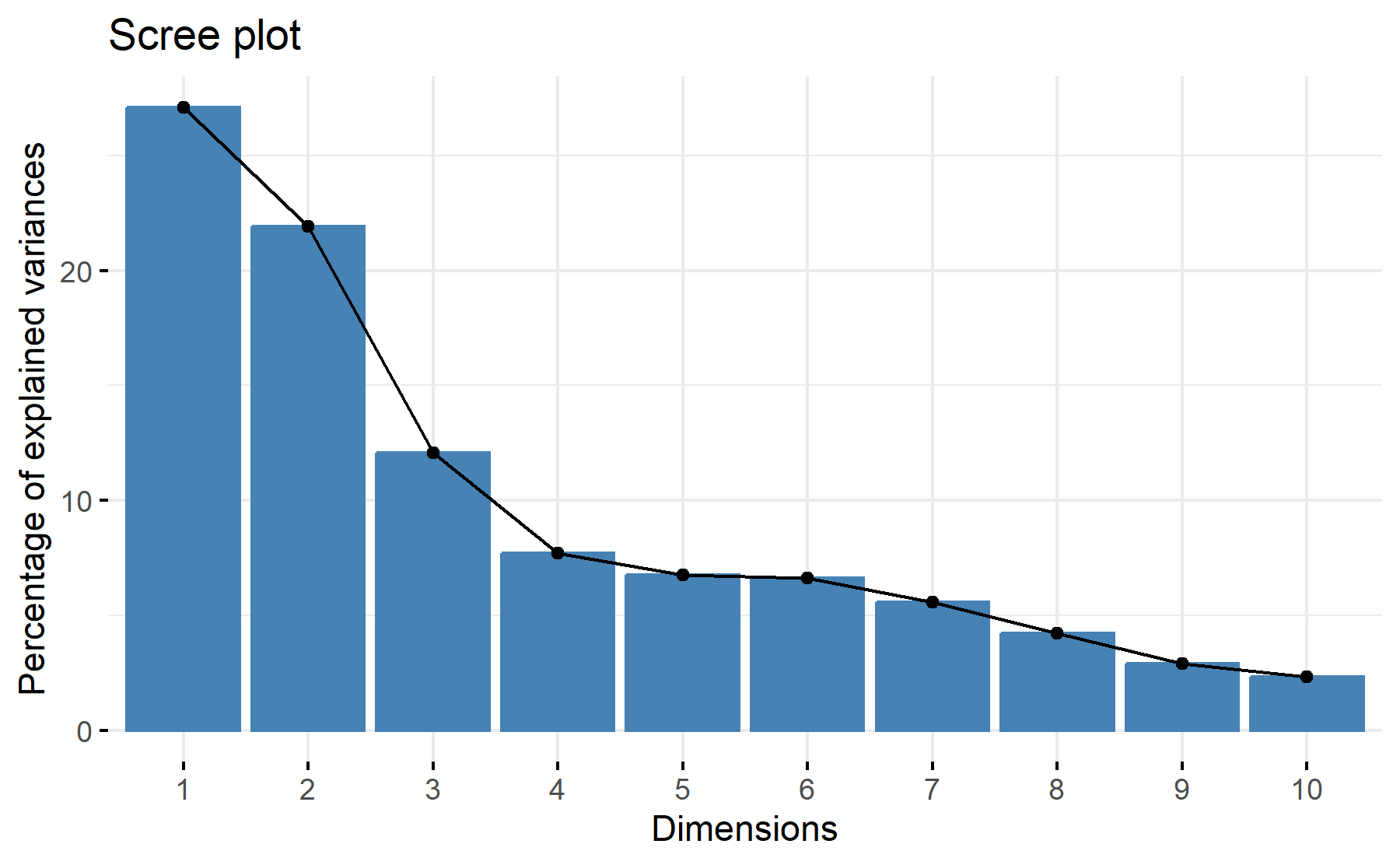
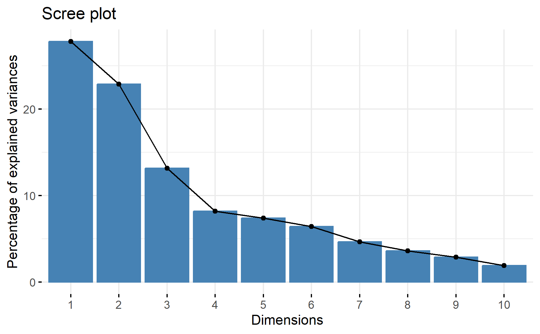
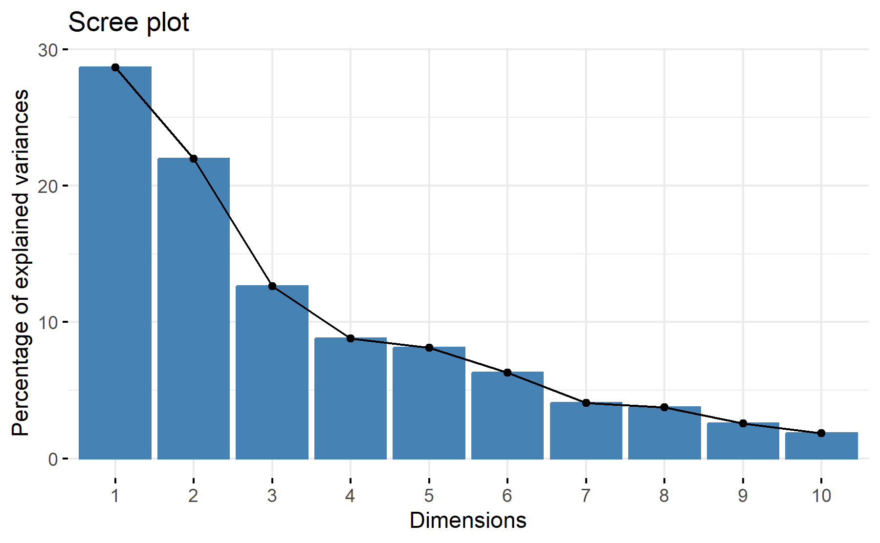
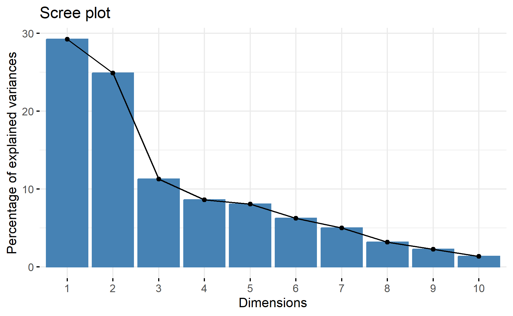
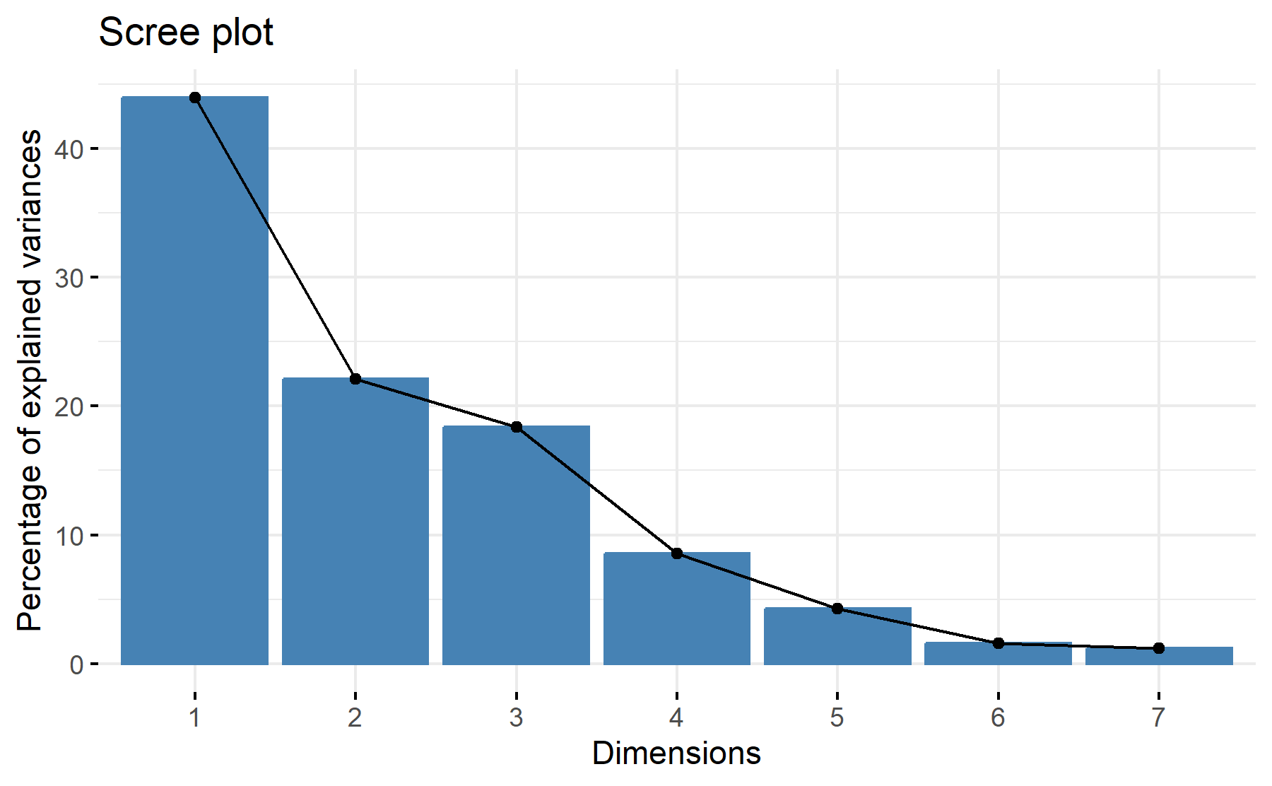
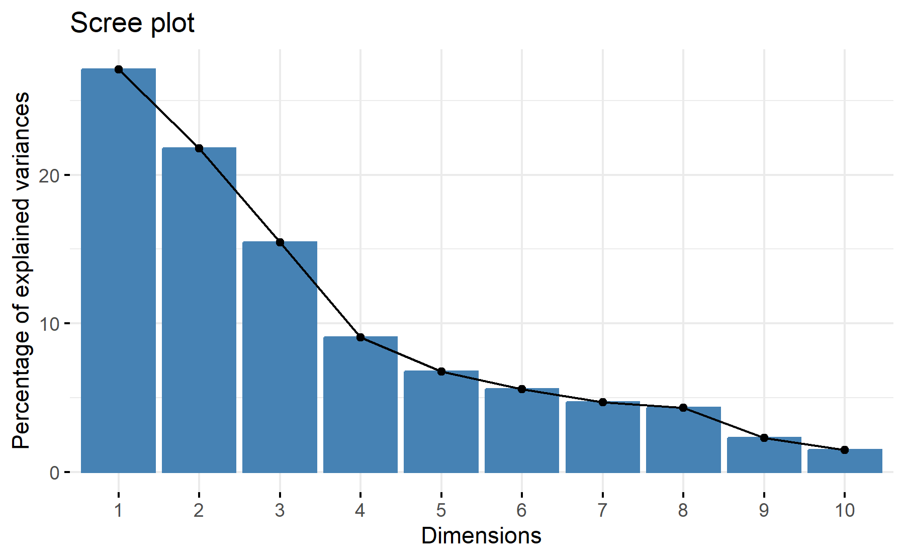
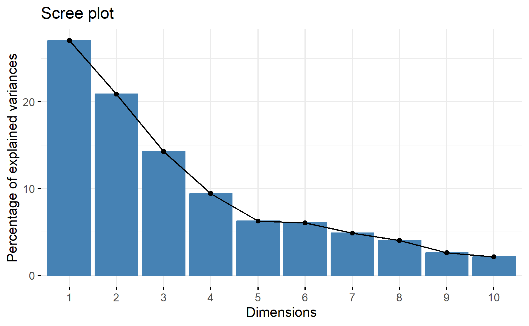
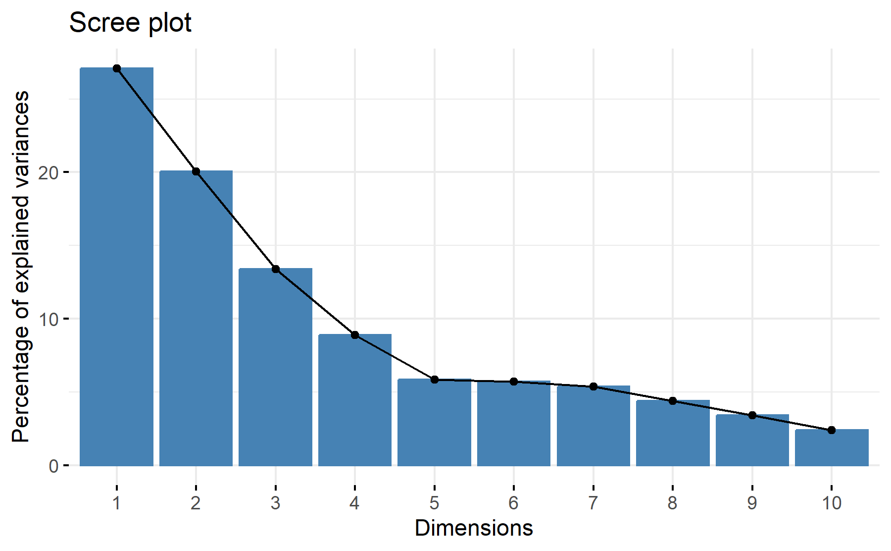
Then, the scree plot for this PCA analysis is displayed.
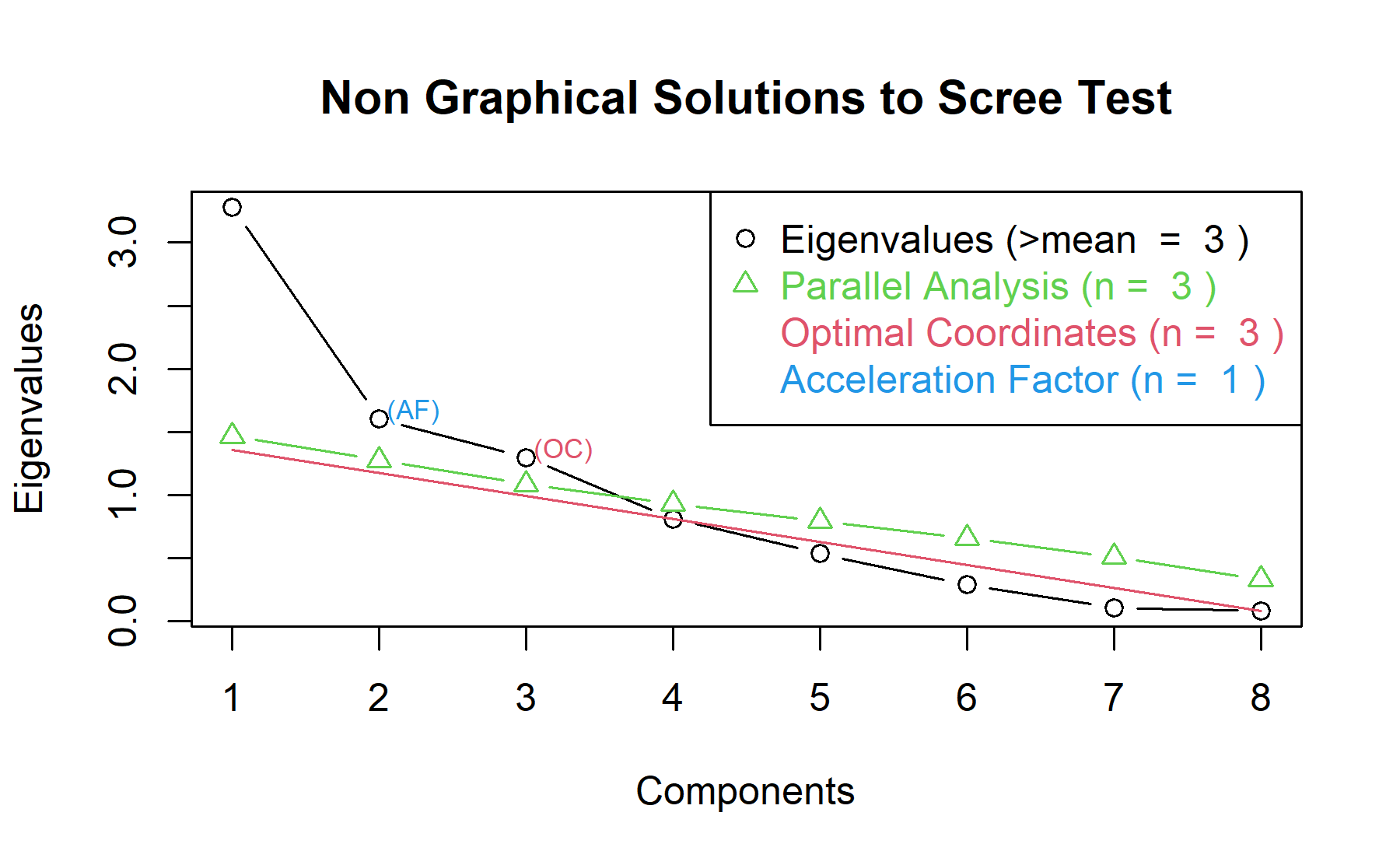
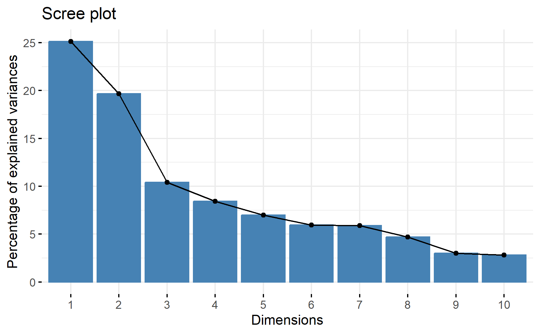 According to these results, 3 factors could be the best number. The cumulative proportion showed that with 3 components 55% of the variance could be explained, besides, just a 8% increase was added with an additional component. While the scree plot exhibit two elbows, the first one after the 2nd component and the other one can be seen after the third one.
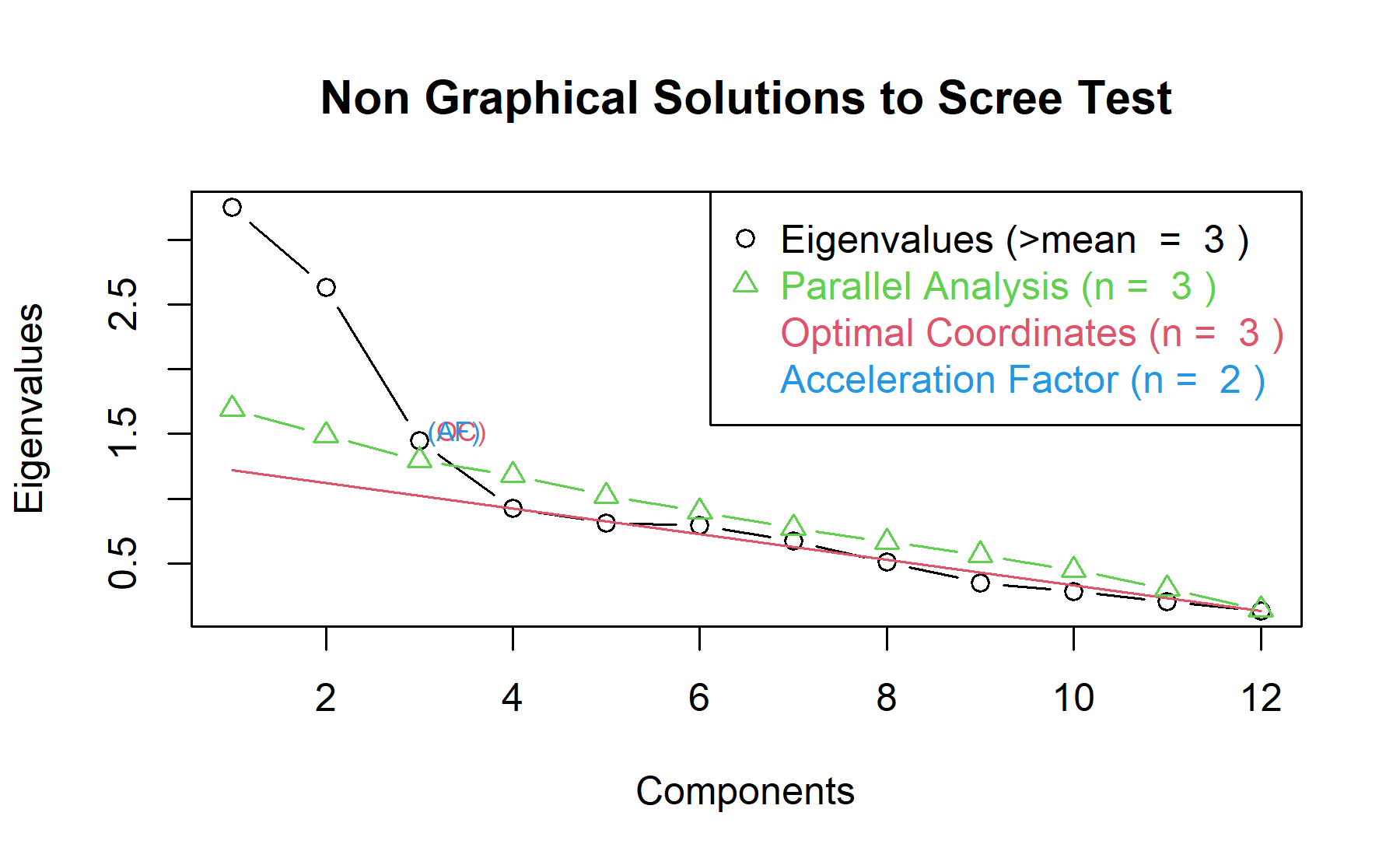
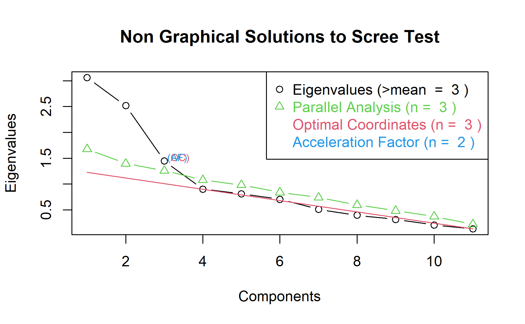
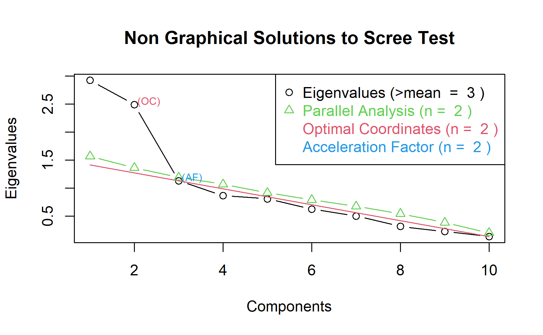
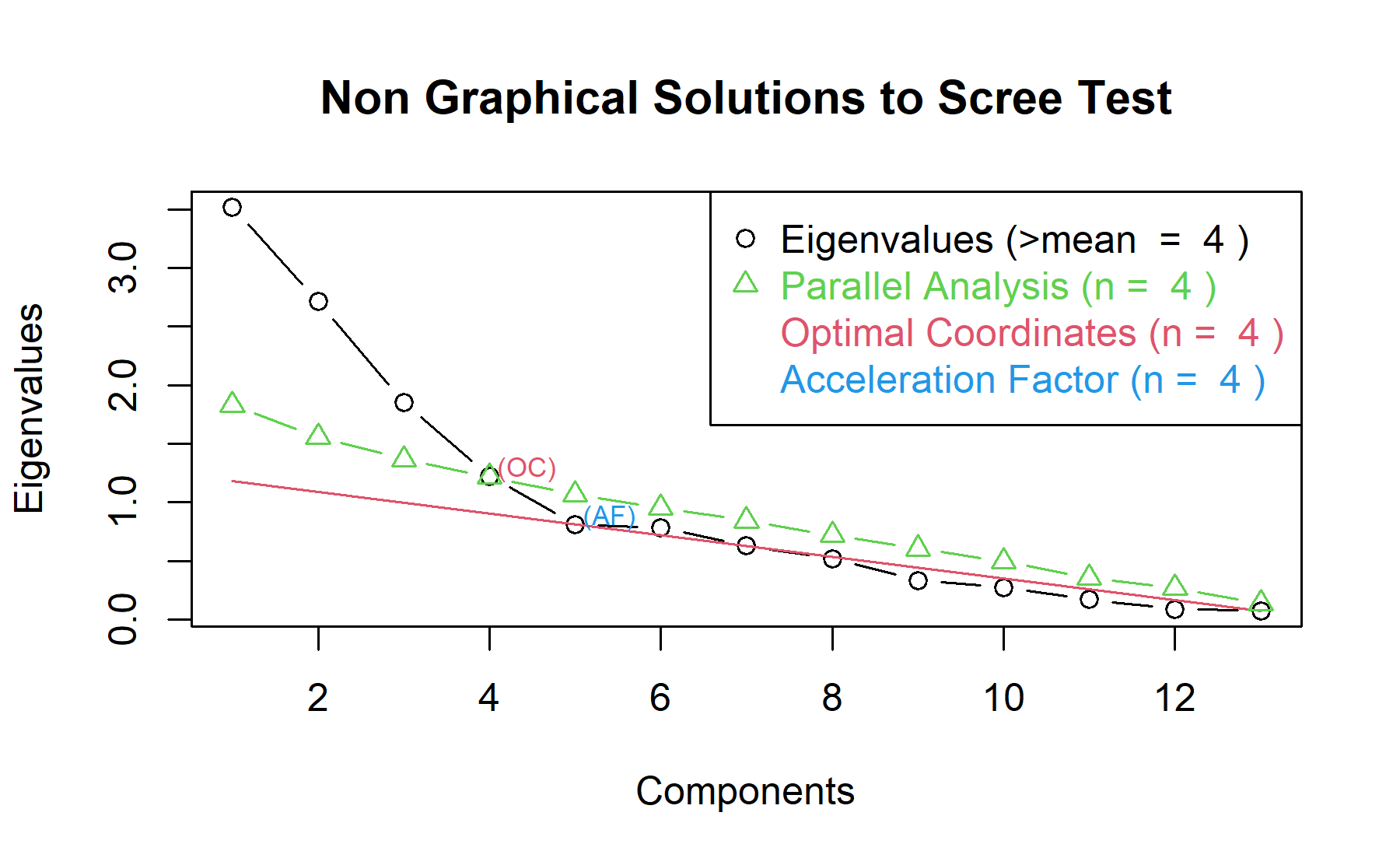
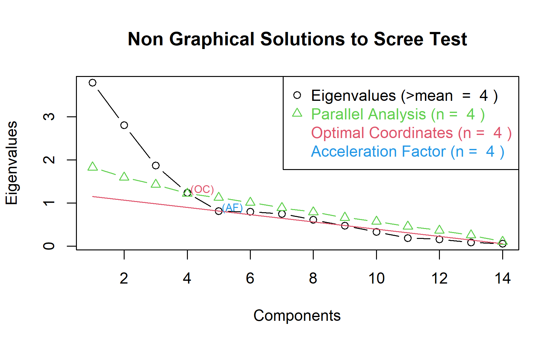
Then, another approach is implemented. With this strategy several analysis are combined and depict in the same figure. The tools implemented are: the Kaiser rule (which drops the components with eigenvalues < 1), the parallel analysis, and the usual scree test (plotuScree), the acceleration factor (which indicates where the elbow of the scree plot appears).
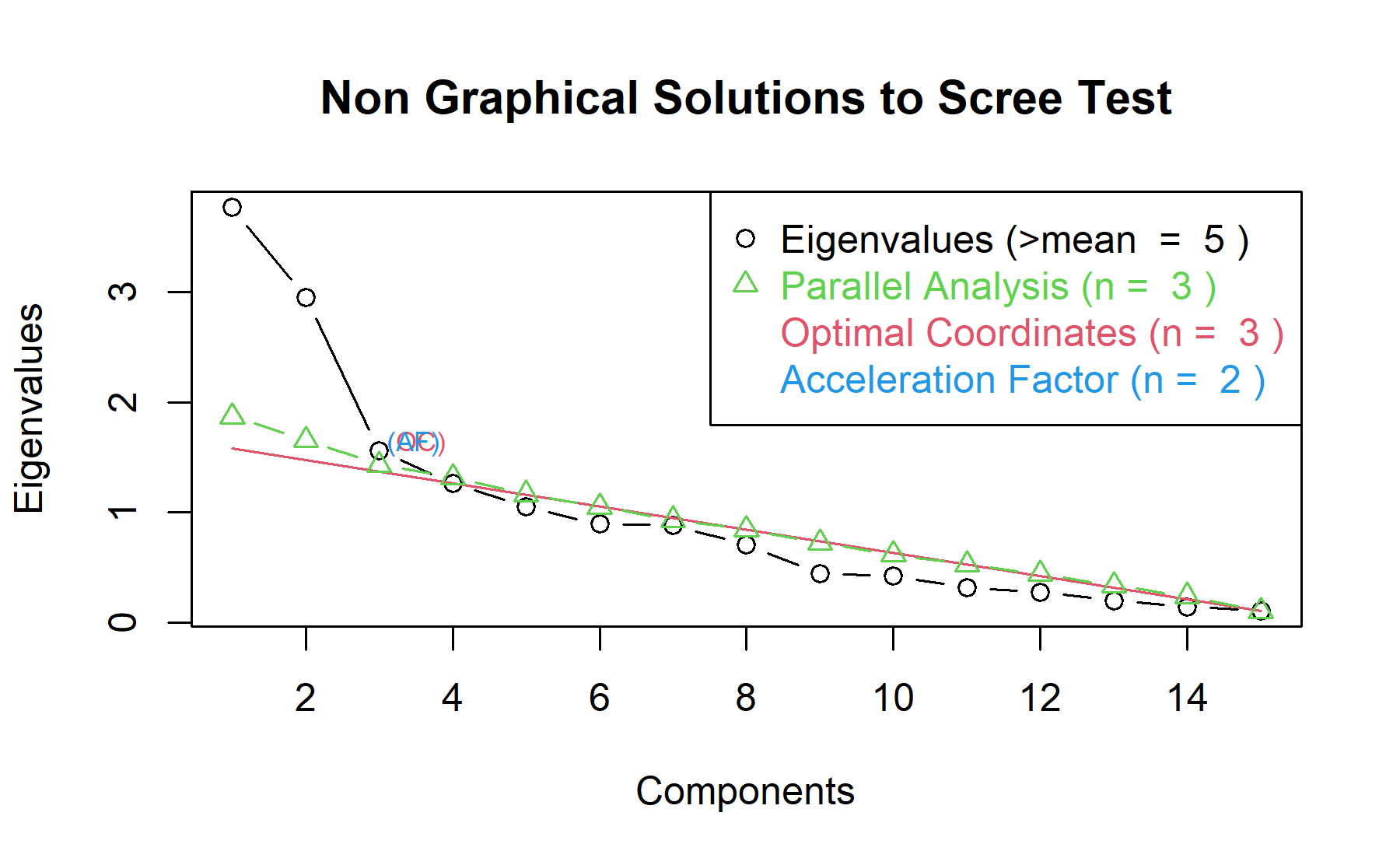 Therefore, considering three factors seem to be an adequate approach.
Running the factor analysis with all the items (n=15), first the communalities are explored:
## Warning in cor.smooth(mat): Matrix was not positive definite, smoothing was
## done
## pre_exp_preoc_q1 pre_exp_preoc_q2 pre_exp_preoc_q3
## 0.84954 0.99500 0.99500
## pre_exp_preoc_q4_Inverted pre_exp_preoc_q5 pre_exp_preoc_q6
## 0.34439 0.36572 0.71030
## pre_exp_preoc_q7_i pre_exp_preoc_q7_ii pre_exp_preoc_q7_iii
## 0.57211 0.02335 0.30293
## pre_exp_preoc_q7_iv pre_exp_preoc_q7_v pre_exp_preoc_q8
## 0.84946 0.97696 0.30218
## pre_exp_preoc_q9 pre_exp_preoc_q10 pre_exp_preoc_q11
## 0.38175 0.20093 0.34393Considering the values of the communalities, item Q7.ii has an extremely lower value. Besides, Q10 showed a value below 0.3. In addition, there are several items with scores between 0.3 and 0.4. Q7.ii has also a lower KMO value.
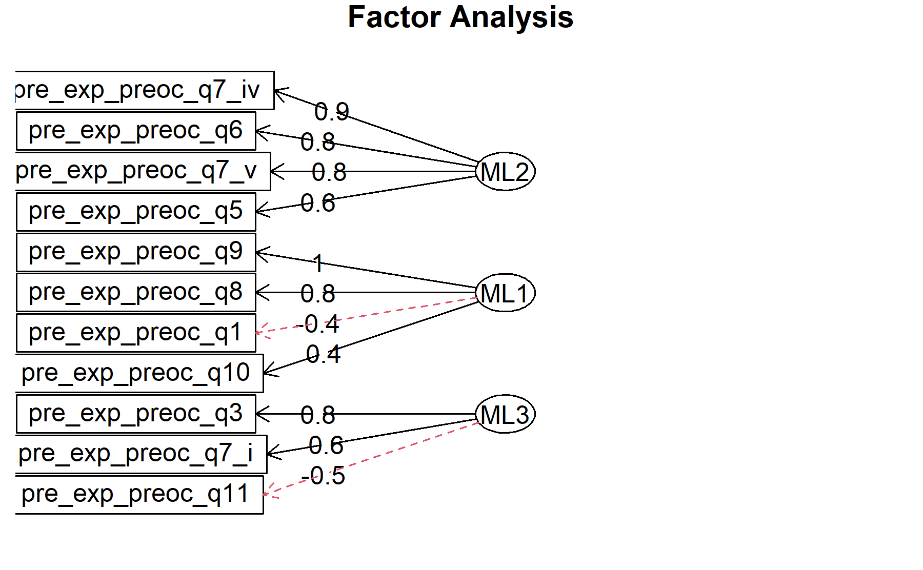
Then, the whole output is displayed.
## Factor Analysis using method = ml
## Call: fa(r = pre_test_Q_ExpConcern_facAn, nfactors = 3, rotate = "oblimin",
## fm = "ml", cor = "poly")
## Standardized loadings (pattern matrix) based upon correlation matrix
## ML2 ML3 ML1 h2 u2 com
## pre_exp_preoc_q1 0.88 0.850 0.1503 1.1
## pre_exp_preoc_q2 1.01 0.995 0.0049 1.0
## pre_exp_preoc_q3 0.97 0.995 0.0050 1.0
## pre_exp_preoc_q4_Inverted 0.59 0.345 0.6547 1.2
## pre_exp_preoc_q5 0.63 0.364 0.6364 1.4
## pre_exp_preoc_q6 0.85 0.711 0.2891 1.1
## pre_exp_preoc_q7_i 0.45 0.48 0.574 0.4258 2.2
## pre_exp_preoc_q7_ii 0.031 0.9686 1.2
## pre_exp_preoc_q7_iii 0.302 0.6978 2.0
## pre_exp_preoc_q7_iv 0.91 0.850 0.1504 1.0
## pre_exp_preoc_q7_v 0.78 0.977 0.0230 1.5
## pre_exp_preoc_q8 -0.54 0.304 0.6961 1.3
## pre_exp_preoc_q9 -0.60 0.380 0.6205 1.1
## pre_exp_preoc_q10 0.200 0.8001 2.6
## pre_exp_preoc_q11 -0.41 0.345 0.6549 2.8
##
## ML2 ML3 ML1
## SS loadings 3.32 2.93 1.97
## Proportion Var 0.22 0.20 0.13
## Cumulative Var 0.22 0.42 0.55
## Proportion Explained 0.40 0.36 0.24
## Cumulative Proportion 0.40 0.76 1.00
##
## With factor correlations of
## ML2 ML3 ML1
## ML2 1.00 0.06 0.15
## ML3 0.06 1.00 0.33
## ML1 0.15 0.33 1.00
##
## Mean item complexity = 1.5
## Test of the hypothesis that 3 factors are sufficient.
##
## df null model = 105 with the objective function = 54.08 with Chi Square = 2172
## df of the model are 63 and the objective function was 45.06
##
## The root mean square of the residuals (RMSR) is 0.12
## The df corrected root mean square of the residuals is 0.15
##
## The harmonic n.obs is 47 with the empirical chi square 139.4 with prob < 0.00000011
## The total n.obs was 47 with Likelihood Chi Square = 1720 with prob < 8.2e-318
##
## Tucker Lewis Index of factoring reliability = -0.41
## RMSEA index = 0.748 and the 90 % confidence intervals are 0.725 0.787
## BIC = 1477
## Fit based upon off diagonal values = 0.88
## Measures of factor score adequacy
## ML2 ML3 ML1
## Correlation of (regression) scores with factors 1.00 0.99 1.00
## Multiple R square of scores with factors 1.00 0.97 0.99
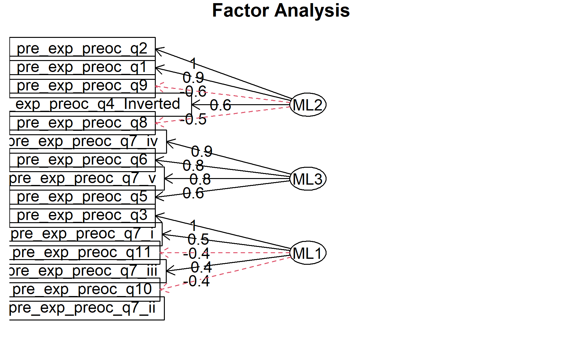
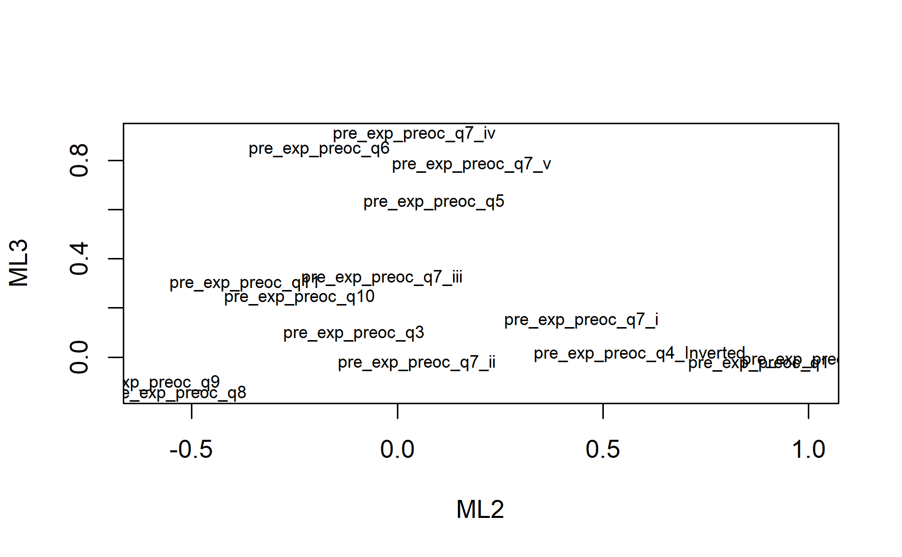
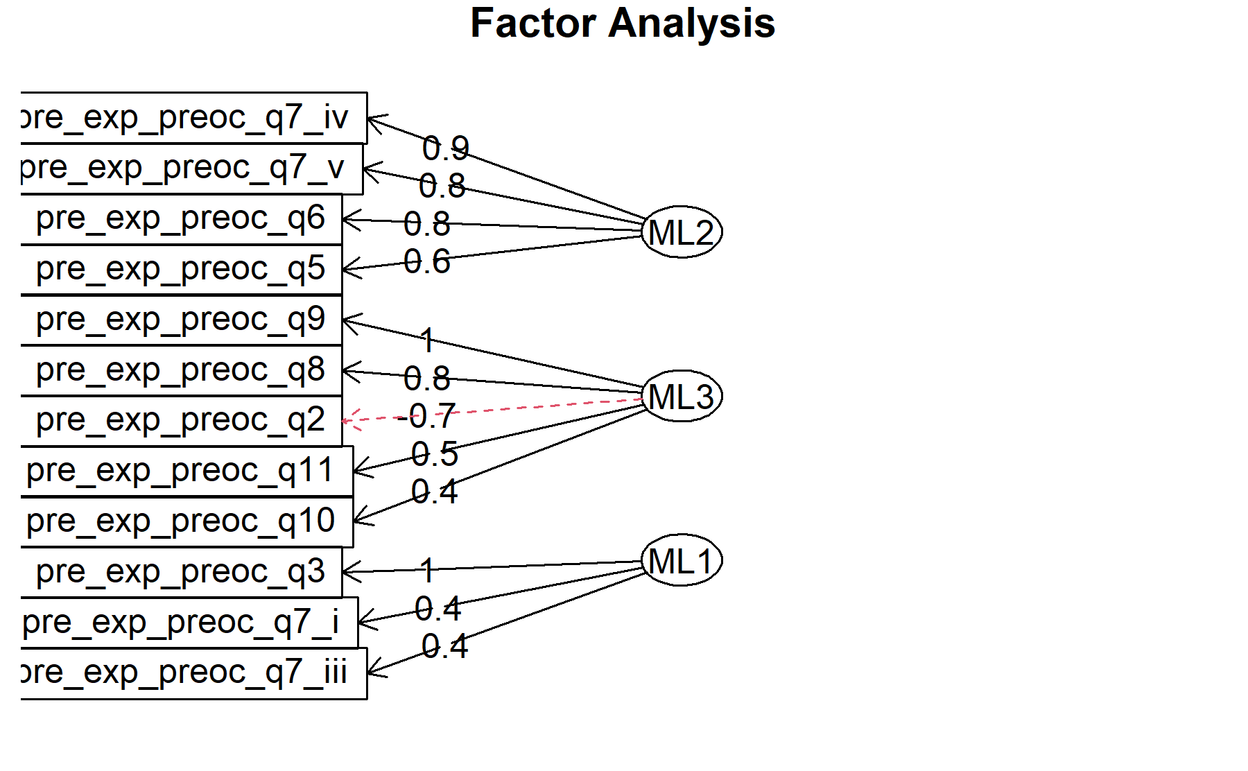
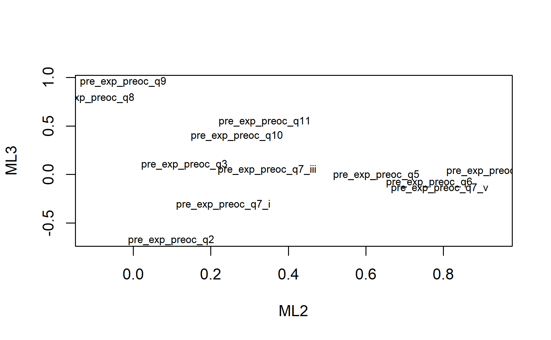
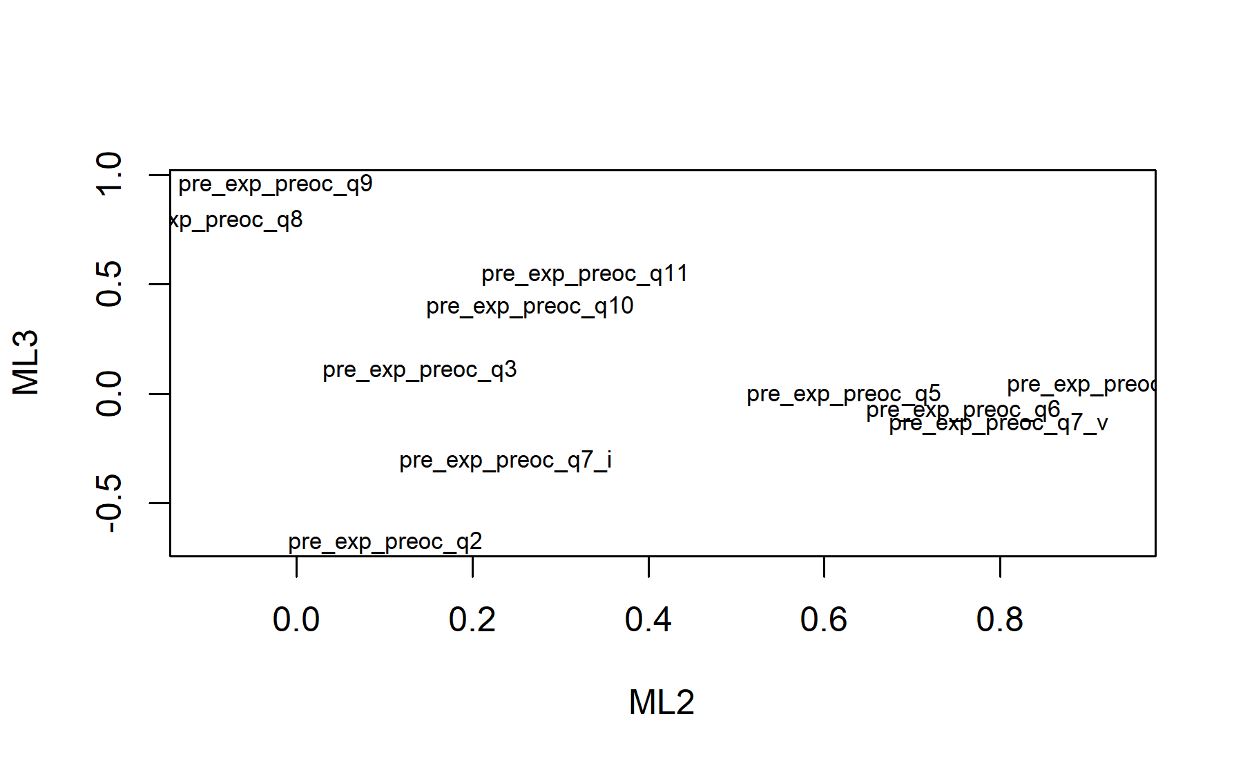
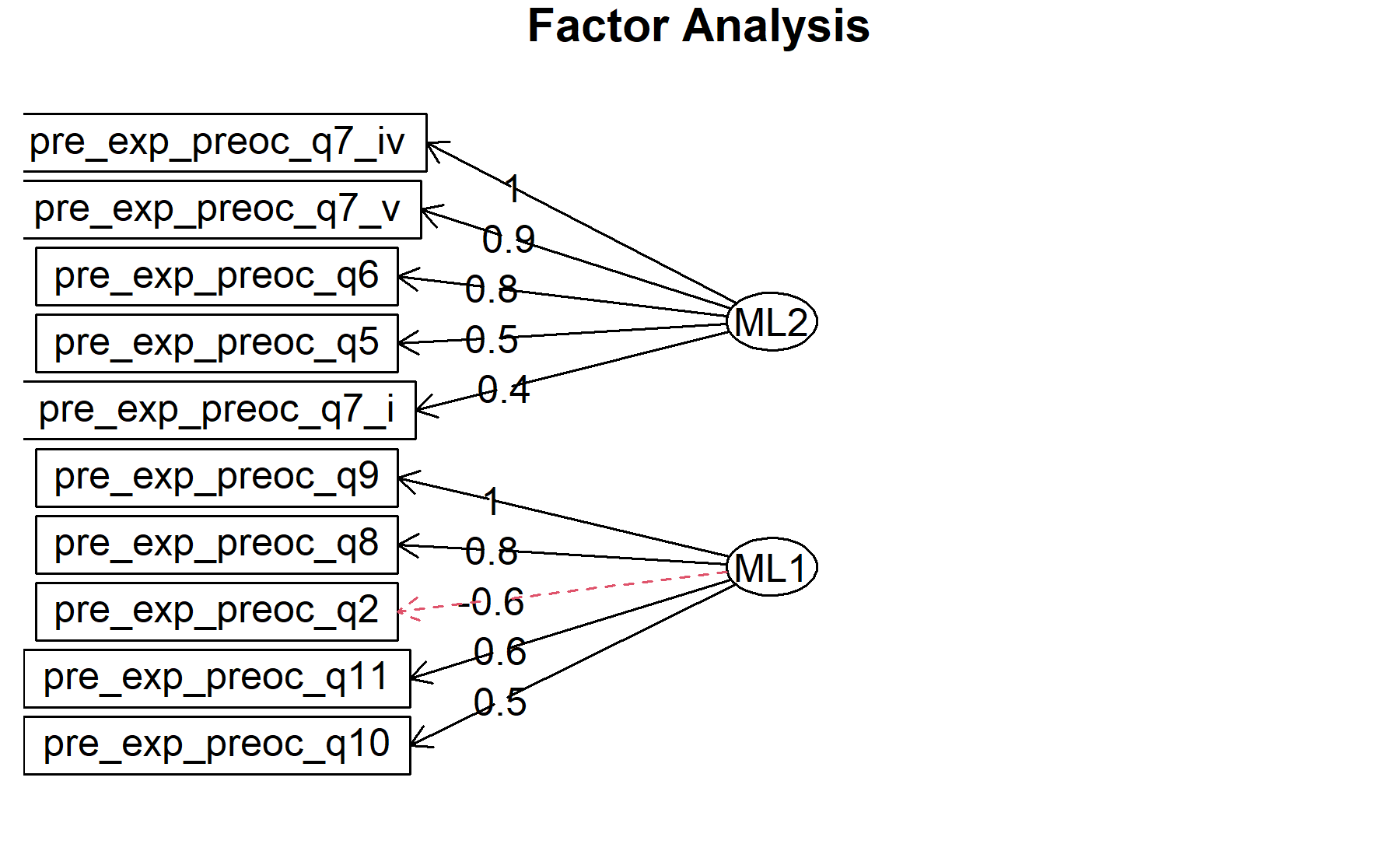
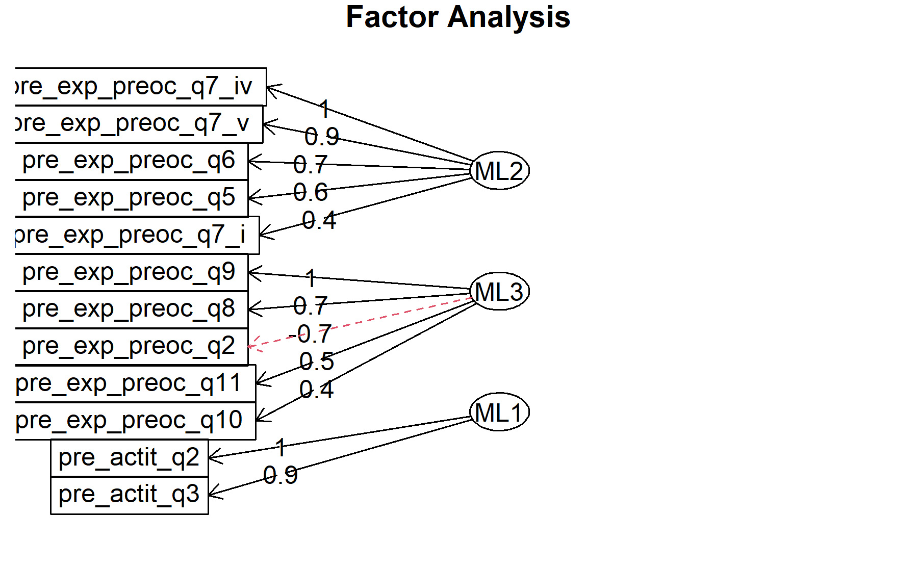
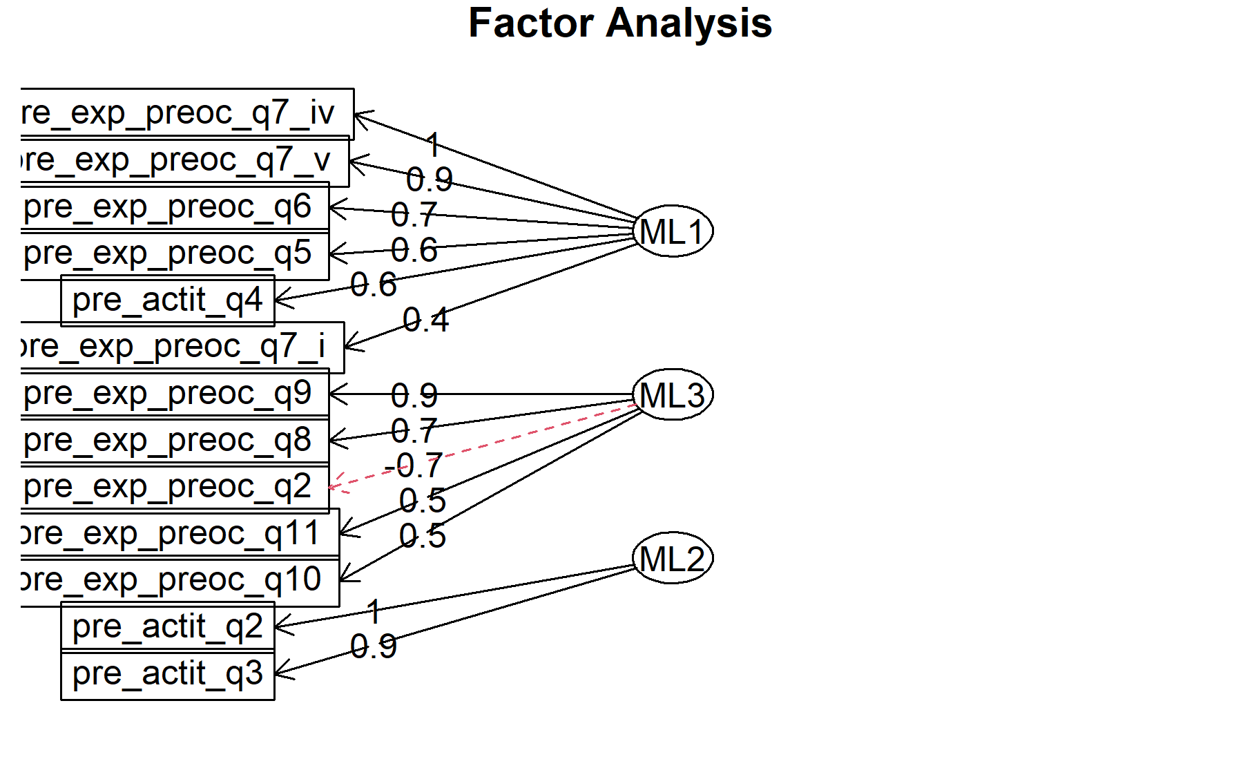
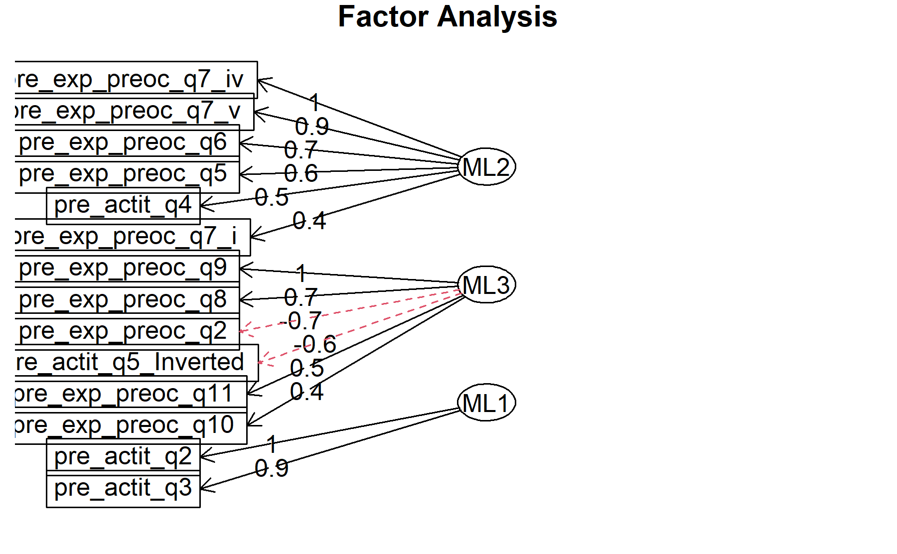
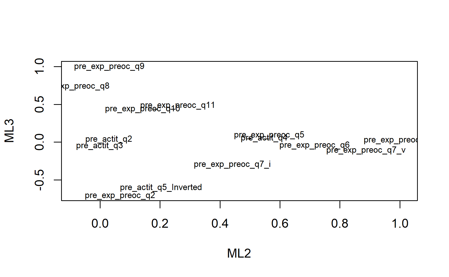
## Minimum correlation of possible factor scores 0.99 0.94 0.99There are 3 factors:
* Q1, Q2, Q4, Q7_i, Q8, Q9.
* Q5, Q6, Q7_iv, Q7_v.
* Q3, Q7_i, Q11.
Out: Q7_ii, Q7_iii
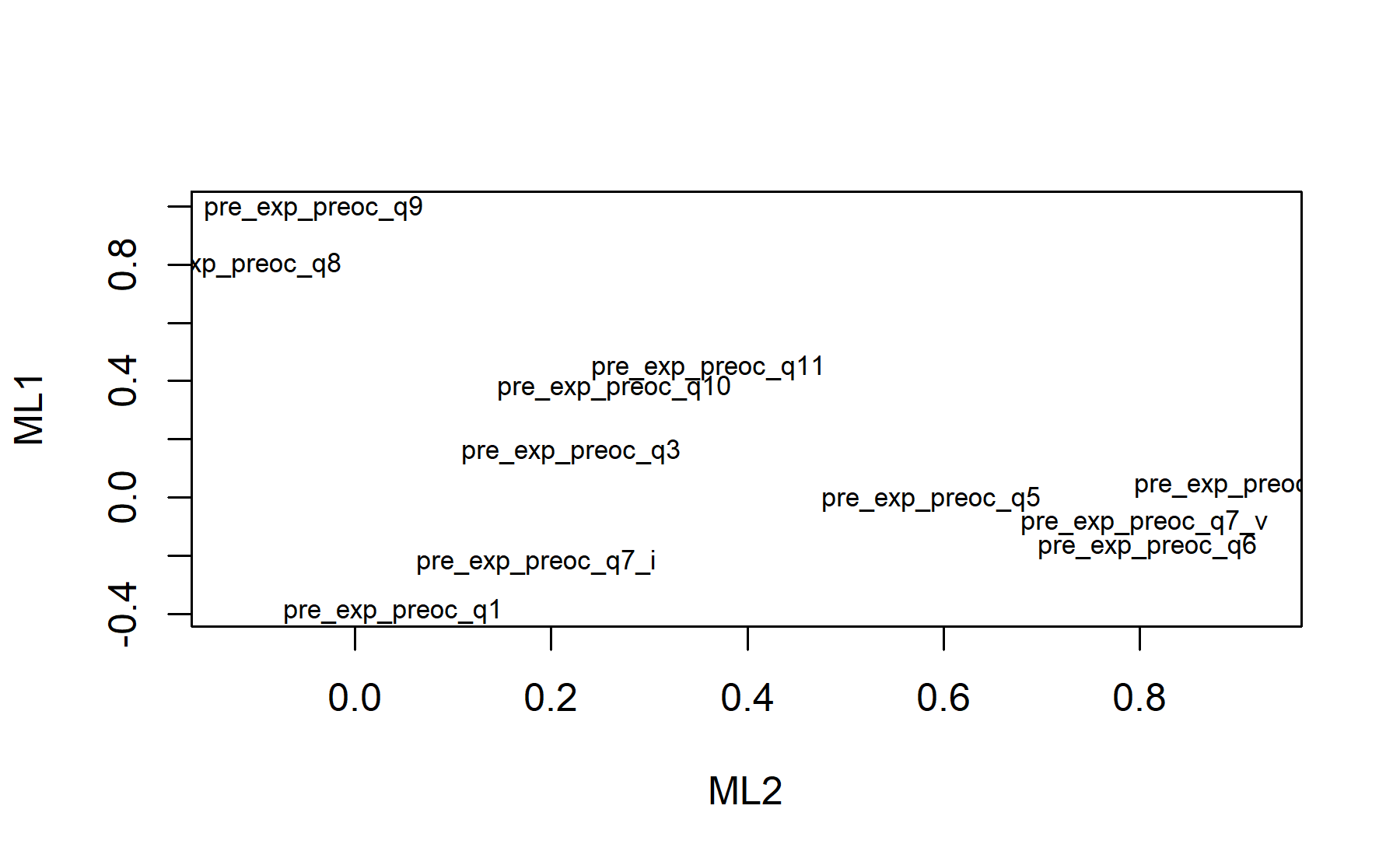
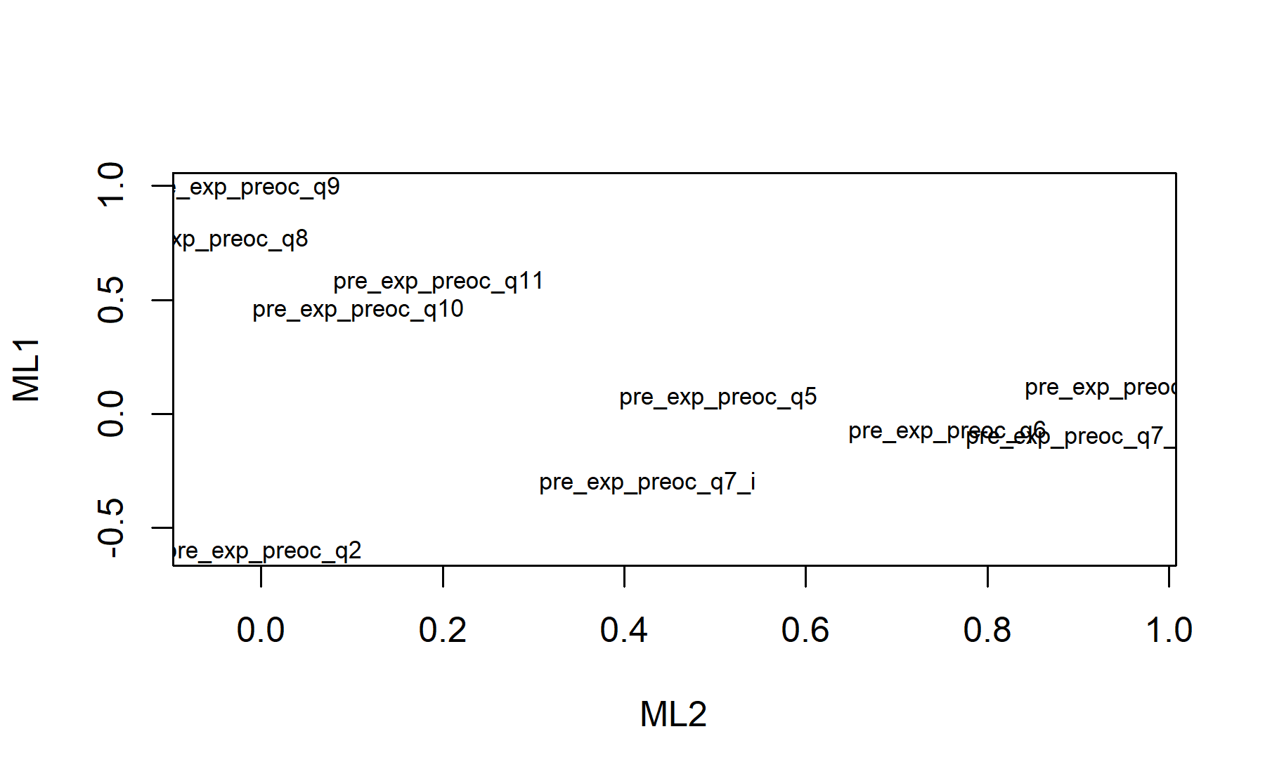
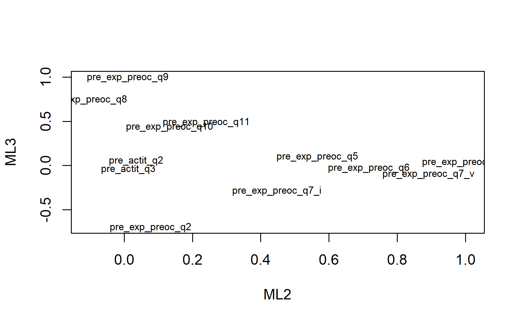
Finally, plots show the relationship between the items and the factors.
10.1.2 Excluding items Q7.ii, Q1, and Q4.
As the first approach, the Q7.ii which showed conflicting results in this dataset, is excluded. Besides, two other items Q1 and Q4 are excluded since they were initially left out.
The Barlett’s sphericity test is performed.
Thus, the p-value = 0 and the H0 is rejected confirming the utility of applying a factor analysis to this dataset.
Considering the fact that the Bartlett’s test usually rejects the H0 since the scenario of the null hypothesis is too extreme, the KMO analysis is studied to determine how well the data fit the factor analysis and how useful each item is.
## Kaiser-Meyer-Olkin factor adequacy
## Call: KMO(r = pre_test_Q_ExpConcern_facAn_2_corr)
## Overall MSA =  0.63
## MSA for each item =
##     q2     q3     q5     q6   q7_i q7_iii  q7_iv   q7_v     q8     q9    q10
##   0.56   0.63   0.51   0.55   0.79   0.70   0.72   0.74   0.58   0.54   0.71
##    q11
##   0.61
According to these results, there is no items under the threshold of 0.5. Five items are below 0.6.
To explore the number of factors PCA is applied. Thus, the table with the PCA results is shown below:
| PC1 | PC2 | PC3 | PC4 | PC5 | PC6 | PC7 | PC8 | PC9 | PC10 | PC11 | PC12 | |
|---|---|---|---|---|---|---|---|---|---|---|---|---|
| Standard deviation | 1.8030 | 1.6222 | 1.2031 | 0.9608 | 0.9011 | 0.8905 | 0.8183 | 0.7126 | 0.5912 | 0.5288 | 0.4505 | 0.3639 |
| Proportion of Variance | 0.2709 | 0.2193 | 0.1206 | 0.0769 | 0.0677 | 0.0661 | 0.0558 | 0.0423 | 0.0291 | 0.0233 | 0.0169 | 0.0110 |
| Cumulative Proportion | 0.2709 | 0.4902 | 0.6108 | 0.6878 | 0.7554 | 0.8215 | 0.8773 | 0.9196 | 0.9487 | 0.9720 | 0.9890 | 1.0000 |
Then, the scree plot for this PCA analysis is displayed.
 According to these results, 3 factors could be the best number. The cumulative proportion showed that with 3 components 61% of the variance could be explained, besides, just a 7% increase was added with an additional component. There is an elbow at the four component.
Then, another approach is implemented. With this strategy several analysis are combined and depict in the same figure. The tools implemented are: the Kaiser rule (which drops the components with eigenvalues < 1), the parallel analysis, and the usual scree test (plotuScree), the acceleration factor (which indicates where the elbow of the scree plot appears).
 Therefore, considering three factors seem to be an adequate approach.
Running the factor analysis with 12 items, first the communalities are explored:
## Warning in cor.smooth(mat): Matrix was not positive definite, smoothing was
## done
## pre_exp_preoc_q2 pre_exp_preoc_q3 pre_exp_preoc_q5
## 0.4603 0.9950 0.3632
## pre_exp_preoc_q6 pre_exp_preoc_q7_i pre_exp_preoc_q7_iii
## 0.5904 0.4682 0.3071
## pre_exp_preoc_q7_iv pre_exp_preoc_q7_v pre_exp_preoc_q8
## 0.8910 0.9632 0.6271
## pre_exp_preoc_q9 pre_exp_preoc_q10 pre_exp_preoc_q11
## 0.9226 0.3255 0.5408Considering the values of the communalities, all are above 0.3. The lowest value can be observed in Q7.iii and Q10.
Then, the whole output is displayed.
## Factor Analysis using method =  ml
## Call: fa(r = pre_test_Q_ExpConcern_facAn_2, nfactors = 3, rotate = "oblimin",
##     fm = "ml", cor = "poly")
## Standardized loadings (pattern matrix) based upon correlation matrix
##                        ML2   ML3   ML1   h2    u2 com
## pre_exp_preoc_q2           -0.68       0.46 0.540 1.2
## pre_exp_preoc_q3                  0.96 1.00 0.005 1.1
## pre_exp_preoc_q5      0.63             0.36 0.637 1.3
## pre_exp_preoc_q6      0.76             0.59 0.410 1.0
## pre_exp_preoc_q7_i                0.45 0.47 0.531 2.3
## pre_exp_preoc_q7_iii                   0.31 0.693 2.0
## pre_exp_preoc_q7_iv   0.94             0.89 0.109 1.0
## pre_exp_preoc_q7_v    0.79             0.96 0.037 1.5
## pre_exp_preoc_q8            0.79       0.63 0.372 1.1
## pre_exp_preoc_q9            0.96       0.92 0.077 1.0
## pre_exp_preoc_q10           0.40       0.33 0.673 2.7
## pre_exp_preoc_q11           0.55 -0.41 0.54 0.459 2.6
##
##                        ML2  ML3  ML1
## SS loadings           2.95 2.63 1.87
## Proportion Var        0.25 0.22 0.16
## Cumulative Var        0.25 0.47 0.62
## Proportion Explained  0.40 0.35 0.25
## Cumulative Proportion 0.40 0.75 1.00
##
##  With factor correlations of
##       ML2   ML3   ML1
## ML2  1.00 -0.08  0.29
## ML3 -0.08  1.00 -0.16
## ML1  0.29 -0.16  1.00
##
## Mean item complexity =  1.6
## Test of the hypothesis that 3 factors are sufficient.
##
## df null model =  66  with the objective function =  30.29 with Chi Square =  1247
## df of  the model are 33  and the objective function was  23.05
##
## The root mean square of the residuals (RMSR) is  0.09
## The df corrected root mean square of the residuals is  0.13
##
## The harmonic n.obs is  47 with the empirical chi square  52.33  with prob <  0.018
## The total n.obs was  47  with Likelihood Chi Square =  902.8  with prob <  2.5e-168
##
## Tucker Lewis Index of factoring reliability =  -0.553
## RMSEA index =  0.749  and the 90 % confidence intervals are  0.715 0.8
## BIC =  775.8
## Fit based upon off diagonal values = 0.94
## Measures of factor score adequacy
##                                                    ML2  ML3  ML1
## Correlation of (regression) scores with factors   0.98 0.97 1.00
## Multiple R square of scores with factors          0.96 0.94 0.99
## Minimum correlation of possible factor scores     0.92 0.88 0.99
There are 3 factors:
* Q2, Q8, Q9, Q10, Q11.
* Q5, Q6, Q7_iv, Q7_v.
* Q3, Q7_i, Q11.
Out: Q7_iii
Finally, plots show the relationship between the items and the factors.
10.1.3 Excluding items Q7.ii, Q1, Q4, and Q7.iii.
Now, the other item with lower scores are excluded (Q7.iii) on top of the previous ones.
The Barlett’s sphericity test is performed.
Thus, the p-value = 0 and the H0 is rejected confirming the utility of applying a factor analysis to this dataset.
Considering the fact that the Bartlett’s test usually rejects the H0 since the scenario of the null hypothesis is too extreme, the KMO analysis is studied to determine how well the data fit the factor analysis and how useful each item is.
## Kaiser-Meyer-Olkin factor adequacy
## Call: KMO(r = pre_test_Q_ExpConcern_facAn_3_corr)
## Overall MSA =  0.61
## MSA for each item =
##    q2    q3    q5    q6  q7_i q7_iv  q7_v    q8    q9   q10   q11
##  0.56  0.65  0.49  0.51  0.78  0.72  0.71  0.61  0.54  0.71  0.62
According to these results, Q5 showed a result of 0.49. Three items are below 0.6.
To explore the number of factors PCA is applied. Thus, the table with the PCA results is shown below:
| PC1 | PC2 | PC3 | PC4 | PC5 | PC6 | PC7 | PC8 | PC9 | PC10 | PC11 | |
|---|---|---|---|---|---|---|---|---|---|---|---|
| Standard deviation | 1.7490 | 1.5862 | 1.2028 | 0.9489 | 0.9008 | 0.8394 | 0.7145 | 0.6291 | 0.5606 | 0.4558 | 0.3655 |
| Proportion of Variance | 0.2781 | 0.2287 | 0.1315 | 0.0819 | 0.0738 | 0.0641 | 0.0464 | 0.0360 | 0.0286 | 0.0189 | 0.0121 |
| Cumulative Proportion | 0.2781 | 0.5068 | 0.6383 | 0.7202 | 0.7940 | 0.8580 | 0.9044 | 0.9404 | 0.9690 | 0.9879 | 1.0000 |
Then, the scree plot for this PCA analysis is displayed.
 According to these results, 3 factors could be the best number. The cumulative proportion showed that with 3 components 64% of the variance could be explained, besides, just a 8% increase was added with an additional component. There is an elbow at the four component.
Then, another approach is implemented. With this strategy several analysis are combined and depict in the same figure. The tools implemented are: the Kaiser rule (which drops the components with eigenvalues < 1), the parallel analysis, and the usual scree test (plotuScree), the acceleration factor (which indicates where the elbow of the scree plot appears).
 Therefore, considering three factors seem to be an adequate approach.
Running the factor analysis with 11 items, first the communalities are explored:
## Warning in cor.smooth(mat): Matrix was not positive definite, smoothing was
## done
## pre_exp_preoc_q2 pre_exp_preoc_q3 pre_exp_preoc_q5 pre_exp_preoc_q6
## 0.4630 0.9950 0.3603 0.5817
## pre_exp_preoc_q7_i pre_exp_preoc_q7_iv pre_exp_preoc_q7_v pre_exp_preoc_q8
## 0.4702 0.8876 0.9686 0.6281
## pre_exp_preoc_q9 pre_exp_preoc_q10 pre_exp_preoc_q11
## 0.9207 0.3265 0.5355Considering the values of the communalities, all are above 0.3. Q10 has the lowest communality value.
Then, the whole output is displayed.
## Factor Analysis using method =  ml
## Call: fa(r = pre_test_Q_ExpConcern_facAn_3, nfactors = 3, rotate = "oblimin",
##     fm = "ml", cor = "poly")
## Standardized loadings (pattern matrix) based upon correlation matrix
##                       ML2   ML3   ML1   h2    u2 com
## pre_exp_preoc_q2          -0.68       0.46 0.536 1.2
## pre_exp_preoc_q3                 0.96 1.00 0.005 1.1
## pre_exp_preoc_q5     0.62             0.36 0.640 1.3
## pre_exp_preoc_q6     0.76             0.58 0.418 1.0
## pre_exp_preoc_q7_i               0.45 0.47 0.530 2.4
## pre_exp_preoc_q7_iv  0.94             0.89 0.113 1.0
## pre_exp_preoc_q7_v   0.80             0.97 0.031 1.4
## pre_exp_preoc_q8           0.79       0.63 0.372 1.1
## pre_exp_preoc_q9           0.96       0.92 0.079 1.0
## pre_exp_preoc_q10          0.40       0.33 0.674 2.7
## pre_exp_preoc_q11          0.55 -0.40 0.54 0.464 2.5
##
##                        ML2  ML3  ML1
## SS loadings           2.79 2.63 1.71
## Proportion Var        0.25 0.24 0.16
## Cumulative Var        0.25 0.49 0.65
## Proportion Explained  0.39 0.37 0.24
## Cumulative Proportion 0.39 0.76 1.00
##
##  With factor correlations of
##       ML2   ML3   ML1
## ML2  1.00 -0.09  0.29
## ML3 -0.09  1.00 -0.17
## ML1  0.29 -0.17  1.00
##
## Mean item complexity =  1.5
## Test of the hypothesis that 3 factors are sufficient.
##
## df null model =  55  with the objective function =  29.28 with Chi Square =  1215
## df of  the model are 25  and the objective function was  22.39
##
## The root mean square of the residuals (RMSR) is  0.09
## The df corrected root mean square of the residuals is  0.13
##
## The harmonic n.obs is  47 with the empirical chi square  38.52  with prob <  0.041
## The total n.obs was  47  with Likelihood Chi Square =  884.6  with prob <  1.7e-170
##
## Tucker Lewis Index of factoring reliability =  -0.717
## RMSEA index =  0.855  and the 90 % confidence intervals are  0.816 0.914
## BIC =  788.3
## Fit based upon off diagonal values = 0.95
## Measures of factor score adequacy
##                                                    ML2  ML3  ML1
## Correlation of (regression) scores with factors   0.98 0.97 1.00
## Multiple R square of scores with factors          0.96 0.94 0.99
## Minimum correlation of possible factor scores     0.93 0.88 0.99
There are 3 factors:
* Q2, Q8, Q9, Q10, Q11.
* Q5, Q6, Q7_iv, Q7_v.
* Q3, Q7_i, Q11.
Finally, plots show the relationship between the items and the factors.

10.1.4 Excluding items Q7.ii, Q2, Q4, and Q7.iii.
Now, the Q1 is changed by Q2 to analyze which of them is the best item to preserve. From the analysis with the first cohort and previous analysis in this cohort, item Q2 seems to be more adequate. However, the factor analysis showed conflicting results in this regard.
The Barlett’s sphericity test is performed.
Thus, the p-value = 0 and the H0 is rejected confirming the utility of applying a factor analysis to this dataset.
Considering the fact that the Bartlett’s test usually rejects the H0 since the scenario of the null hypothesis is too extreme, the KMO analysis is studied to determine how well the data fit the factor analysis and how useful each item is.
## Kaiser-Meyer-Olkin factor adequacy
## Call: KMO(r = pre_test_Q_ExpConcern_facAn_4_corr)
## Overall MSA =  0.61
## MSA for each item =
##    q1    q3    q5    q6  q7_i q7_iv  q7_v    q8    q9   q10   q11
##  0.54  0.68  0.46  0.52  0.70  0.72  0.71  0.59  0.54  0.68  0.60
According to these results, Q5 showed a result of 0.46. Four items are below 0.6.
To explore the number of factors PCA is applied. Thus, the table with the PCA results is shown below:
| PC1 | PC2 | PC3 | PC4 | PC5 | PC6 | PC7 | PC8 | PC9 | PC10 | PC11 | |
|---|---|---|---|---|---|---|---|---|---|---|---|
| Standard deviation | 1.7755 | 1.5541 | 1.1789 | 0.9827 | 0.9445 | 0.8316 | 0.6701 | 0.6430 | 0.5331 | 0.4527 | 0.3765 |
| Proportion of Variance | 0.2866 | 0.2196 | 0.1264 | 0.0878 | 0.0811 | 0.0629 | 0.0408 | 0.0376 | 0.0258 | 0.0186 | 0.0129 |
| Cumulative Proportion | 0.2866 | 0.5061 | 0.6325 | 0.7203 | 0.8014 | 0.8642 | 0.9051 | 0.9426 | 0.9685 | 0.9871 | 1.0000 |
Then, the scree plot for this PCA analysis is displayed.
 Now it is less clear, could be 3 factors, but 2 or 4 seem to be useful as well. The cumulative proportion for 3 components is 63% and for four component 72%. The elbow is located at the four component.
Then, another approach is implemented. With this strategy several analysis are combined and depict in the same figure. The tools implemented are: the Kaiser rule (which drops the components with eigenvalues < 1), the parallel analysis, and the usual scree test (plotuScree), the acceleration factor (which indicates where the elbow of the scree plot appears).
 Therefore, considering three factors seem to be an adequate approach.
Running the factor analysis with 11 items, first the communalities are explored:
## Warning in cor.smooth(mat): Matrix was not positive definite, smoothing was
## done
## pre_exp_preoc_q1 pre_exp_preoc_q3 pre_exp_preoc_q5 pre_exp_preoc_q6
## 0.3208 0.7841 0.3216 0.6506
## pre_exp_preoc_q7_i pre_exp_preoc_q7_iv pre_exp_preoc_q7_v pre_exp_preoc_q8
## 0.5114 0.8736 0.9945 0.6249
## pre_exp_preoc_q9 pre_exp_preoc_q10 pre_exp_preoc_q11
## 0.9950 0.3371 0.6170Considering the values of the communalities, all are above 0.3. Q10 has the lowest communality value.
Then, the whole output is displayed.
## Factor Analysis using method =  ml
## Call: fa(r = pre_test_Q_ExpConcern_facAn_4, nfactors = 3, rotate = "oblimin",
##     fm = "ml", cor = "poly")
## Standardized loadings (pattern matrix) based upon correlation matrix
##                       ML2   ML1   ML3   h2     u2 com
## pre_exp_preoc_q1                      0.32 0.6790 1.9
## pre_exp_preoc_q3                 0.83 0.78 0.2159 1.2
## pre_exp_preoc_q5     0.59             0.32 0.6771 1.1
## pre_exp_preoc_q6     0.81             0.65 0.3499 1.1
## pre_exp_preoc_q7_i               0.56 0.51 0.4890 1.5
## pre_exp_preoc_q7_iv  0.92             0.87 0.1263 1.0
## pre_exp_preoc_q7_v   0.80             0.99 0.0055 1.5
## pre_exp_preoc_q8           0.80       0.62 0.3756 1.1
## pre_exp_preoc_q9           1.00       1.00 0.0050 1.0
## pre_exp_preoc_q10                     0.34 0.6632 2.8
## pre_exp_preoc_q11          0.45 -0.53 0.62 0.3832 2.7
##
##                        ML2  ML1  ML3
## SS loadings           2.84 2.34 1.85
## Proportion Var        0.26 0.21 0.17
## Cumulative Var        0.26 0.47 0.64
## Proportion Explained  0.40 0.33 0.26
## Cumulative Proportion 0.40 0.74 1.00
##
##  With factor correlations of
##       ML2   ML1   ML3
## ML2  1.00 -0.06  0.25
## ML1 -0.06  1.00 -0.25
## ML3  0.25 -0.25  1.00
##
## Mean item complexity =  1.6
## Test of the hypothesis that 3 factors are sufficient.
##
## df null model =  55  with the objective function =  29.4 with Chi Square =  1220
## df of  the model are 25  and the objective function was  22.58
##
## The root mean square of the residuals (RMSR) is  0.09
## The df corrected root mean square of the residuals is  0.13
##
## The harmonic n.obs is  47 with the empirical chi square  40.59  with prob <  0.025
## The total n.obs was  47  with Likelihood Chi Square =  891.9  with prob <  4.6e-172
##
## Tucker Lewis Index of factoring reliability =  -0.724
## RMSEA index =  0.859  and the 90 % confidence intervals are  0.82 0.918
## BIC =  795.7
## Fit based upon off diagonal values = 0.94
## Measures of factor score adequacy
##                                                    ML2  ML1  ML3
## Correlation of (regression) scores with factors   0.98 1.00 0.94
## Multiple R square of scores with factors          0.97 0.99 0.88
## Minimum correlation of possible factor scores     0.94 0.99 0.77
There are 3 factors:
* Q8, Q9, Q11.
* Q5, Q6, Q7_iv, Q7_v.
* Q3, Q7_i, Q11.
Out: Q10
Finally, plots show the relationship between the items and the factors.
Changing Q2 by Q1, the latter showed a lower communality value and it did not appear in any factor when the threshold was set in 0.4.
10.1.5 Excluding items Q7_ii, Q1, and Q4, plus Q7_iii and Q3.
The first three items seem to be conflicting and with no relevant information. On the other hand, Q7_iii and Q3 are collecting interesting data but probably they are not related with the other questions in a particular domain. Therefore, these could be excluded from the factor analysis but they could be retained inside the questionnaire.

The Barlett’s sphericity test is performed.
Thus, the p-value = 0 and the H0 is rejected confirming the utility of applying a factor analysis to this dataset.
Considering the fact that the Bartlett’s test usually rejects the H0 since the scenario of the null hypothesis is too extreme, the KMO analysis is studied to determine how well the data fit the factor analysis and how useful each item is.
## Kaiser-Meyer-Olkin factor adequacy
## Call: KMO(r = pre_test_Q_ExpConcern_facAn_5_corr)
## Overall MSA =  0.59
## MSA for each item =
##    q2    q5    q6  q7_i q7_iv  q7_v    q8    q9   q10   q11
##  0.56  0.49  0.50  0.76  0.68  0.69  0.60  0.53  0.68  0.60
According to these results, there is one items under the threshold of 0.5 (Q5=0.49). Three items are below 0.6.
To explore the number of factors PCA is applied. Thus, the table with the PCA results is shown below:
| PC1 | PC2 | PC3 | PC4 | PC5 | PC6 | PC7 | PC8 | PC9 | PC10 | |
|---|---|---|---|---|---|---|---|---|---|---|
| Standard deviation | 1.7092 | 1.5773 | 1.0622 | 0.9283 | 0.8981 | 0.7891 | 0.7071 | 0.5609 | 0.4729 | 0.3655 |
| Proportion of Variance | 0.2921 | 0.2488 | 0.1128 | 0.0862 | 0.0807 | 0.0623 | 0.0500 | 0.0315 | 0.0224 | 0.0134 |
| Cumulative Proportion | 0.2921 | 0.5409 | 0.6537 | 0.7399 | 0.8206 | 0.8828 | 0.9328 | 0.9643 | 0.9866 | 1.0000 |
Then, the scree plot for this PCA analysis is displayed.
 According to these results, 2-3 factors could be the best number. The cumulative proportion showed that with 3 components 65% but the greatest elbow appeared after the second component the four component.
Then, another approach is implemented. With this strategy several analysis are combined and depict in the same figure. The tools implemented are: the Kaiser rule (which drops the components with eigenvalues < 1), the parallel analysis, and the usual scree test (plotuScree), the acceleration factor (which indicates where the elbow of the scree plot appears).
 Therefore, considering two factors seem to be an adequate approach.
Running the factor analysis with 10 items, first the communalities are explored:
## Warning in cor.smooth(mat): Matrix was not positive definite, smoothing was
## done
## pre_exp_preoc_q2 pre_exp_preoc_q5 pre_exp_preoc_q6 pre_exp_preoc_q7_i
## 0.3632 0.2472 0.5962 0.3132
## pre_exp_preoc_q7_iv pre_exp_preoc_q7_v pre_exp_preoc_q8 pre_exp_preoc_q9
## 0.9129 0.8472 0.6033 0.9950
## pre_exp_preoc_q10 pre_exp_preoc_q11
## 0.2056 0.3397Considering the values of the communalities, Q5 and Q10 are below 0.3.
Then, the whole output is displayed.
## Factor Analysis using method =  ml
## Call: fa(r = pre_test_Q_ExpConcern_facAn_5, nfactors = 2, rotate = "oblimin",
##     fm = "ml", cor = "poly")
## Standardized loadings (pattern matrix) based upon correlation matrix
##                       ML2   ML1   h2    u2 com
## pre_exp_preoc_q2          -0.60 0.36 0.636 1.0
## pre_exp_preoc_q5     0.50       0.25 0.752 1.0
## pre_exp_preoc_q6     0.76       0.60 0.404 1.0
## pre_exp_preoc_q7_i   0.43       0.31 0.687 1.8
## pre_exp_preoc_q7_iv  0.97       0.91 0.087 1.0
## pre_exp_preoc_q7_v   0.90       0.85 0.153 1.0
## pre_exp_preoc_q8           0.77 0.60 0.396 1.0
## pre_exp_preoc_q9           0.99 1.00 0.005 1.0
## pre_exp_preoc_q10          0.46 0.21 0.795 1.1
## pre_exp_preoc_q11          0.58 0.34 0.660 1.2
##
##                        ML2  ML1
## SS loadings           2.81 2.61
## Proportion Var        0.28 0.26
## Cumulative Var        0.28 0.54
## Proportion Explained  0.52 0.48
## Cumulative Proportion 0.52 1.00
##
##  With factor correlations of
##       ML2   ML1
## ML2  1.00 -0.16
## ML1 -0.16  1.00
##
## Mean item complexity =  1.1
## Test of the hypothesis that 2 factors are sufficient.
##
## df null model =  45  with the objective function =  27.55 with Chi Square =  1153
## df of  the model are 26  and the objective function was  22.58
##
## The root mean square of the residuals (RMSR) is  0.12
## The df corrected root mean square of the residuals is  0.16
##
## The harmonic n.obs is  47 with the empirical chi square  61.79  with prob <  0.000096
## The total n.obs was  47  with Likelihood Chi Square =  914.6  with prob <  4.5e-176
##
## Tucker Lewis Index of factoring reliability =  -0.436
## RMSEA index =  0.852  and the 90 % confidence intervals are  0.815 0.91
## BIC =  814.5
## Fit based upon off diagonal values = 0.9
## Measures of factor score adequacy
##                                                    ML2  ML1
## Correlation of (regression) scores with factors   0.97 1.00
## Multiple R square of scores with factors          0.95 1.00
## Minimum correlation of possible factor scores     0.90 0.99
There are 2 factors:
* Q2, Q8, Q9, Q10, Q11.
* Q5, Q6, Q7_i, Q7_iv, Q7_v.
Finally, plots show the relationship between the items and the factors.
10.2 Attitudes domain
In this setting, again, the goal is to compare the results of this cohort to those from the VHIO cohort maintaining the same principles.
Regarding this domain the global idea is to exclude motivation items and only preserve the question that allows the patient to select the main motivation. Thus, from the six items studied one should be excluded (candidates items 4 or 5 from the pre and post genomic testing questionnaire). Considering the pre genomic testing results, item 5 seems to be the worst of them.
First, a factor analysis with all the 8 items is performed, then two more will be applied one without item 4 and other without item 5.
10.2.1 All the items (n=8).
First, a factor analysis with all the 8 items is performed.
As first approach the Barlett’s sphericity test is performed.
Thus, the p-value = 0 and the H0 is rejected confirming the utility of applying a factor analysis to this dataset.
Considering the fact that the Bartlett’s test usually rejects the H0 since the scenario of the null hypothesis is too extreme, the KMO analysis is studied to determine how well the data fit the factor analysis and how useful each item is.
## Kaiser-Meyer-Olkin factor adequacy
## Call: KMO(r = pre_test_Q_Actitd_facAn_1_corr)
## Overall MSA = 0.58
## MSA for each item =
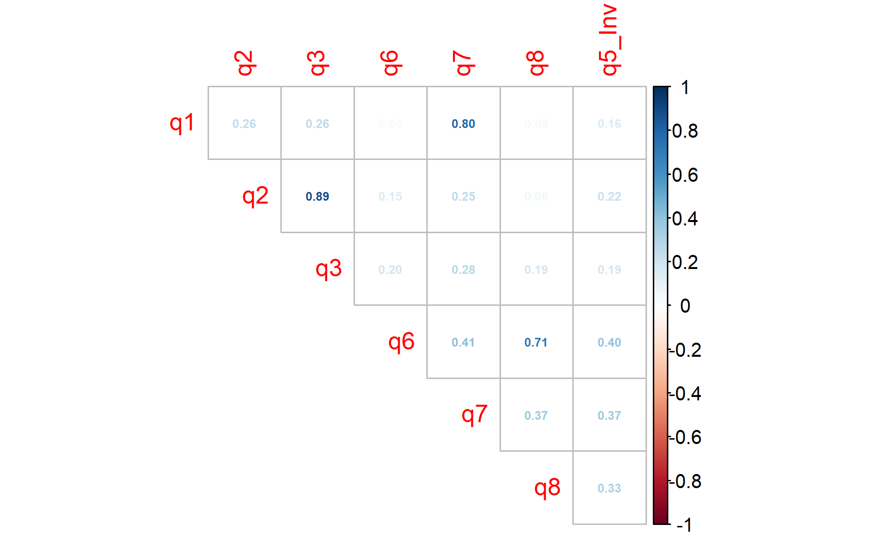
## q1 q2 q3 q4 q6 q7 q8 q5_Inv
## 0.49 0.51 0.53 0.65 0.62 0.60 0.61 0.78According to these results, there is one items under the threshold of 0.5 (Q1=0.49). Two items are below 0.6.
To explore the number of factors PCA and evaluate the variability explained for each component is considered. Thus, the table with the PCA results is shown below:
| PC1 | PC2 | PC3 | PC4 | PC5 | PC6 | PC7 | PC8 | |
|---|---|---|---|---|---|---|---|---|
| Standard deviation | 1.8105 | 1.2659 | 1.1386 | 0.9006 | 0.7315 | 0.5367 | 0.3252 | 0.2879 |
| Proportion of Variance | 0.4098 | 0.2003 | 0.1621 | 0.1014 | 0.0669 | 0.0360 | 0.0132 | 0.0104 |
| Cumulative Proportion | 0.4098 | 0.6101 | 0.7721 | 0.8735 | 0.9404 | 0.9764 | 0.9896 | 1.0000 |
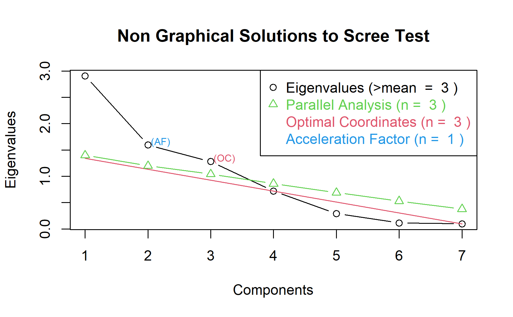
Then, the scree plot for this PCA analysis is displayed.
 According to these results, with two 61% of the variability is explained and with three 77%. And two elbows could be identified, the first one clearly on the second component, and another one on the thrid component.
Then, another approach is implemented. With this strategy several analysis are combined and depict in the same figure. The tools implemented are: the Kaiser rule (which drops the components with eigenvalues < 1), the parallel analysis, and the usual scree test (plotuScree), the acceleration factor (which indicates where the elbow of the scree plot appears).
 Therefore, three factors will be considered.
Running the factor analysis with all the items (n=8), first the communalities are explored:
## Warning in cor.smooth(mat): Matrix was not positive definite, smoothing was
## done
## pre_actit_q1 pre_actit_q2 pre_actit_q3
## 0.9950 0.9950 0.8630
## pre_actit_q4 pre_actit_q6 pre_actit_q7
## 0.7682 0.9950 0.8541
## pre_actit_q8 pre_actit_q5_Inverted
## 0.8575 0.3752Therefore, considering the values of the communalities, only the Q5 inverted is under 0.4.
Then, the whole output is displayed.
## Factor Analysis using method = ml
## Call: fa(r = pre_test_Q_Actitd_facAn_1, nfactors = 3, rotate = "oblimin",
## fm = "ml", cor = "poly")
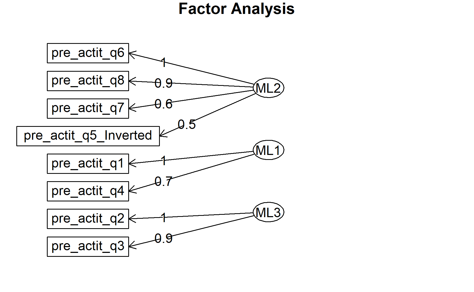
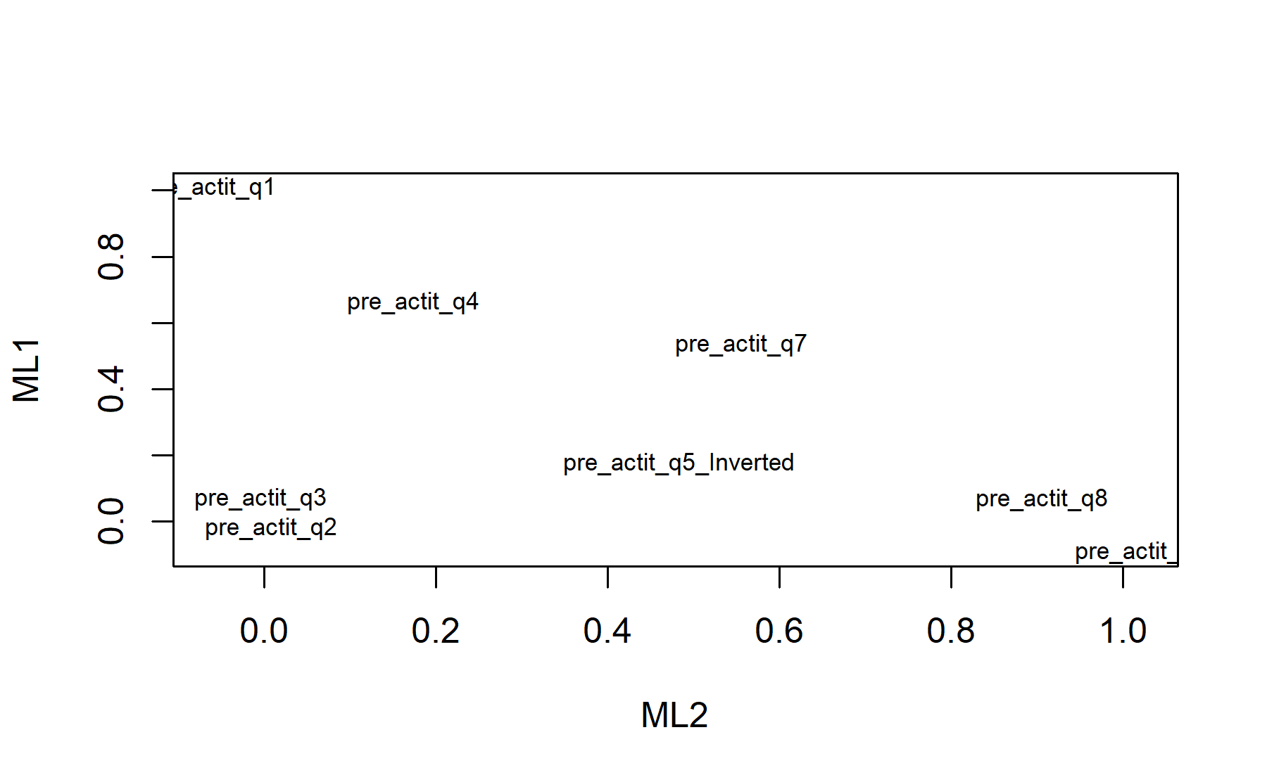
## Standardized loadings (pattern matrix) based upon correlation matrix
## ML2 ML1 ML3 h2 u2 com
## pre_actit_q1 1.01 1.00 0.0049 1.0
## pre_actit_q2 1.00 1.00 0.0049 1.0
## pre_actit_q3 0.89 0.86 0.1370 1.0
## pre_actit_q4 0.66 0.77 0.2318 1.3
## pre_actit_q6 1.02 1.00 0.0050 1.0
## pre_actit_q7 0.56 0.53 0.85 0.1459 2.0
## pre_actit_q8 0.91 0.86 0.1425 1.0
## pre_actit_q5_Inverted 0.48 0.38 0.6247 1.3
##
## ML2 ML1 ML3
## SS loadings 2.66 2.08 1.96
## Proportion Var 0.33 0.26 0.25
## Cumulative Var 0.33 0.59 0.84
## Proportion Explained 0.40 0.31 0.29
## Cumulative Proportion 0.40 0.71 1.00
##
## With factor correlations of
## ML2 ML1 ML3
## ML2 1.00 0.52 0.25
## ML1 0.52 1.00 0.48
## ML3 0.25 0.48 1.00
##
## Mean item complexity = 1.2
## Test of the hypothesis that 3 factors are sufficient.
##
## df null model = 28 with the objective function = 29.11 with Chi Square = 1237
## df of the model are 7 and the objective function was 20.88
##
## The root mean square of the residuals (RMSR) is 0.06
## The df corrected root mean square of the residuals is 0.12
##
## The harmonic n.obs is 47 with the empirical chi square 9.37 with prob < 0.23
## The total n.obs was 47 with Likelihood Chi Square = 845.7 with prob < 2.5e-178
##
## Tucker Lewis Index of factoring reliability = -1.915
## RMSEA index = 1.597 and the 90 % confidence intervals are 1.523 1.707
## BIC = 818.8
## Fit based upon off diagonal values = 0.99
## Measures of factor score adequacy
## ML2 ML1 ML3
## Correlation of (regression) scores with factors 1.00 1.00 1.00
## Multiple R square of scores with factors 1.00 1.00 1.00
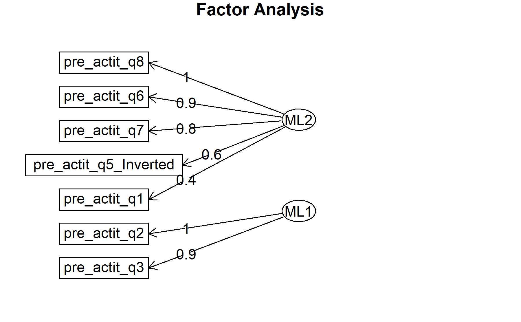
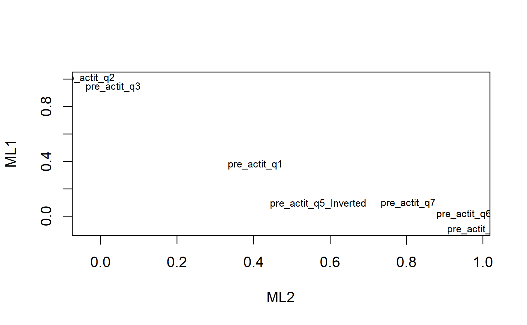
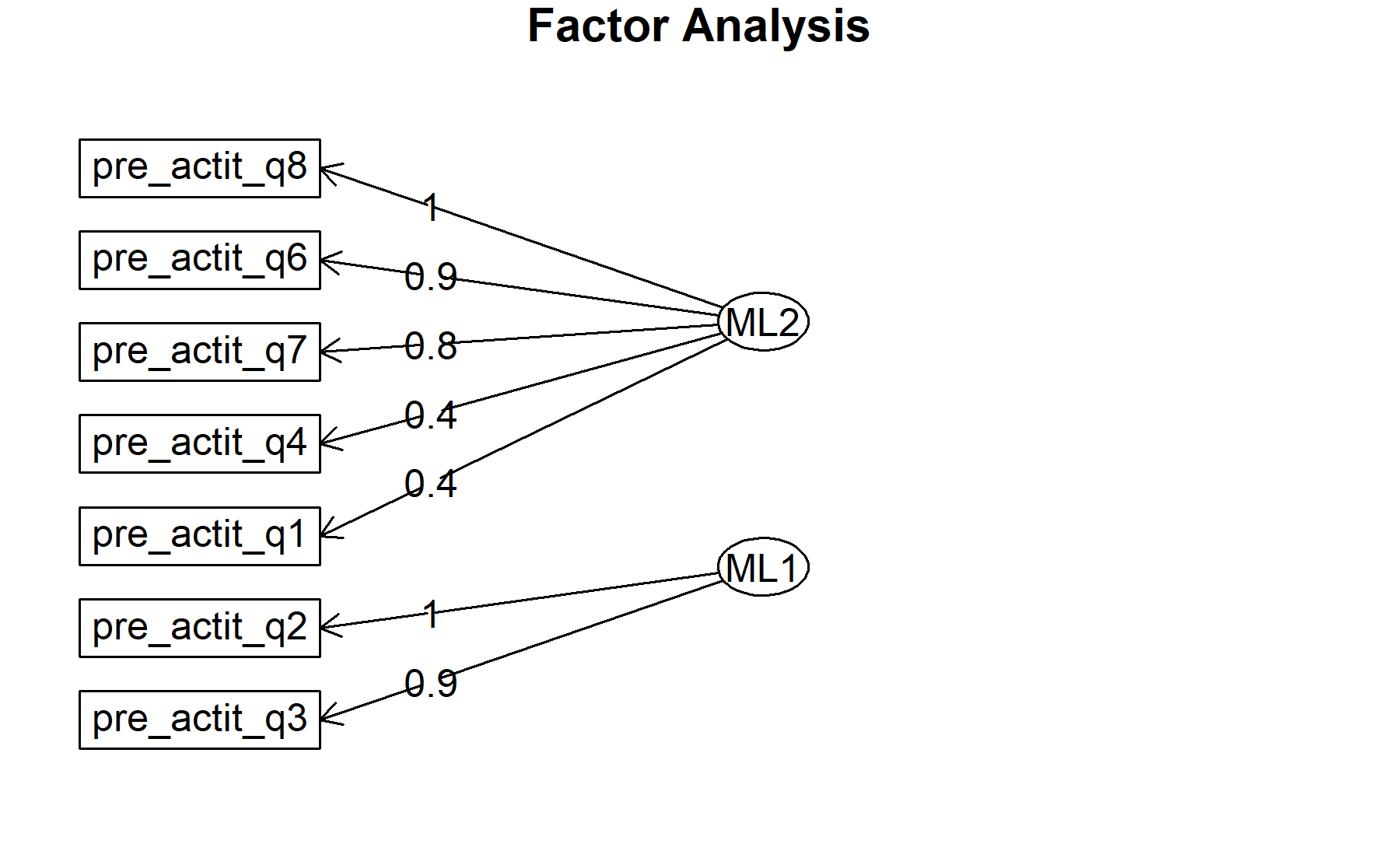
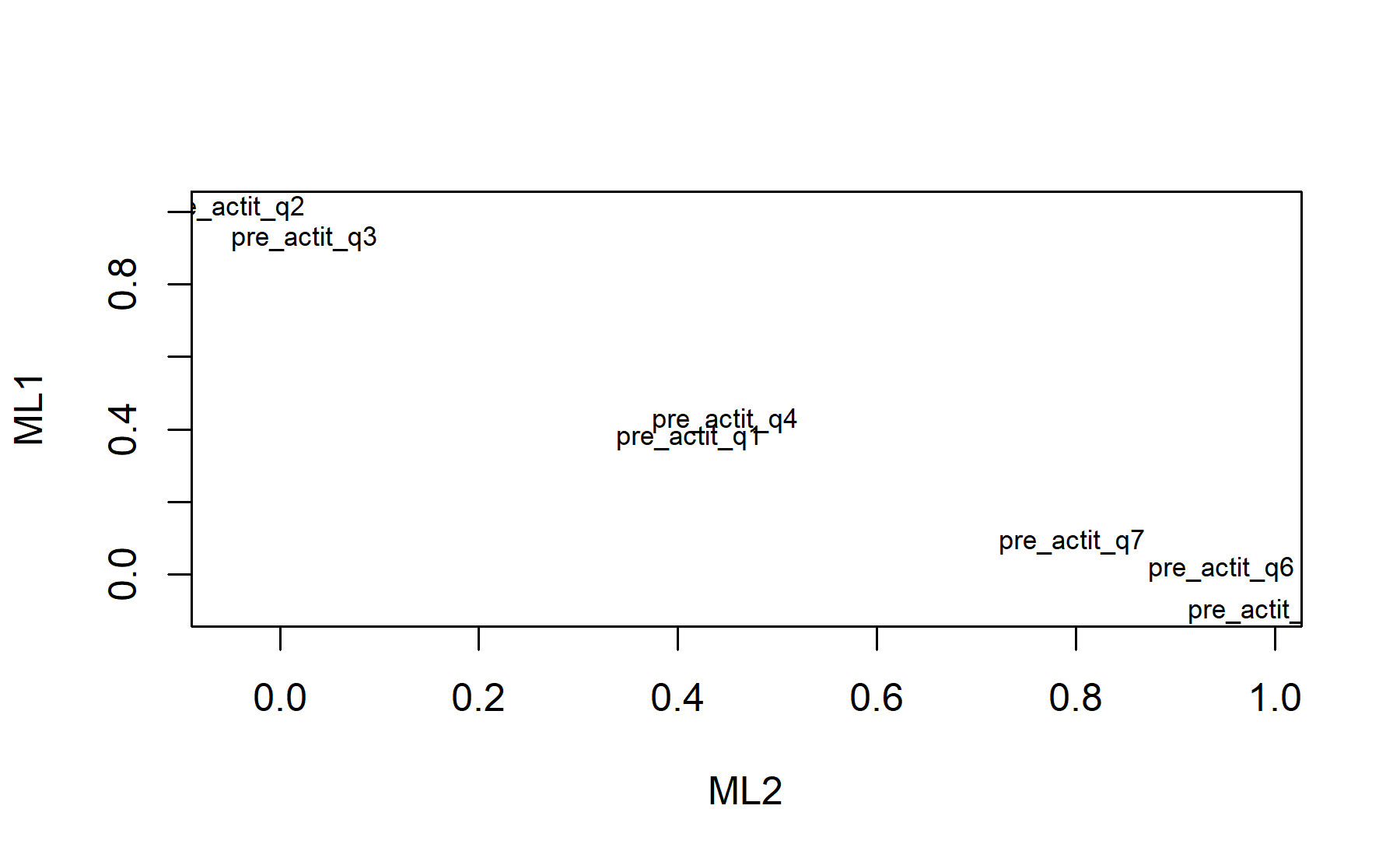
## Minimum correlation of possible factor scores 0.99 0.99 0.99Exploring these results, there are two factors composed by:
* Q6, Q7, Q8, and Q5 inv.
* Q1, Q4, and Q7.
* Q2, and Q3.
Finally, plots show the relationship between the items and the factors.
Then, another factor analysis is run but considering only two factors.
Running the factor analysis with all the items (n=8), first the communalities are explored:
## Warning in cor.smooth(mat): Matrix was not positive definite, smoothing was
## done
## pre_actit_q1 pre_actit_q2 pre_actit_q3
## 0.4240 0.9950 0.8616
## pre_actit_q4 pre_actit_q6 pre_actit_q7
## 0.5025 0.9095 0.7153
## pre_actit_q8 pre_actit_q5_Inverted
## 0.8972 0.3650Therefore, considering the values of the communalities, only the Q5 inverted is under 0.4.
Then, the whole output is displayed.
## Factor Analysis using method = ml
## Call: fa(r = pre_test_Q_Actitd_facAn_1, nfactors = 2, rotate = "oblimin",
## fm = "ml", cor = "poly")
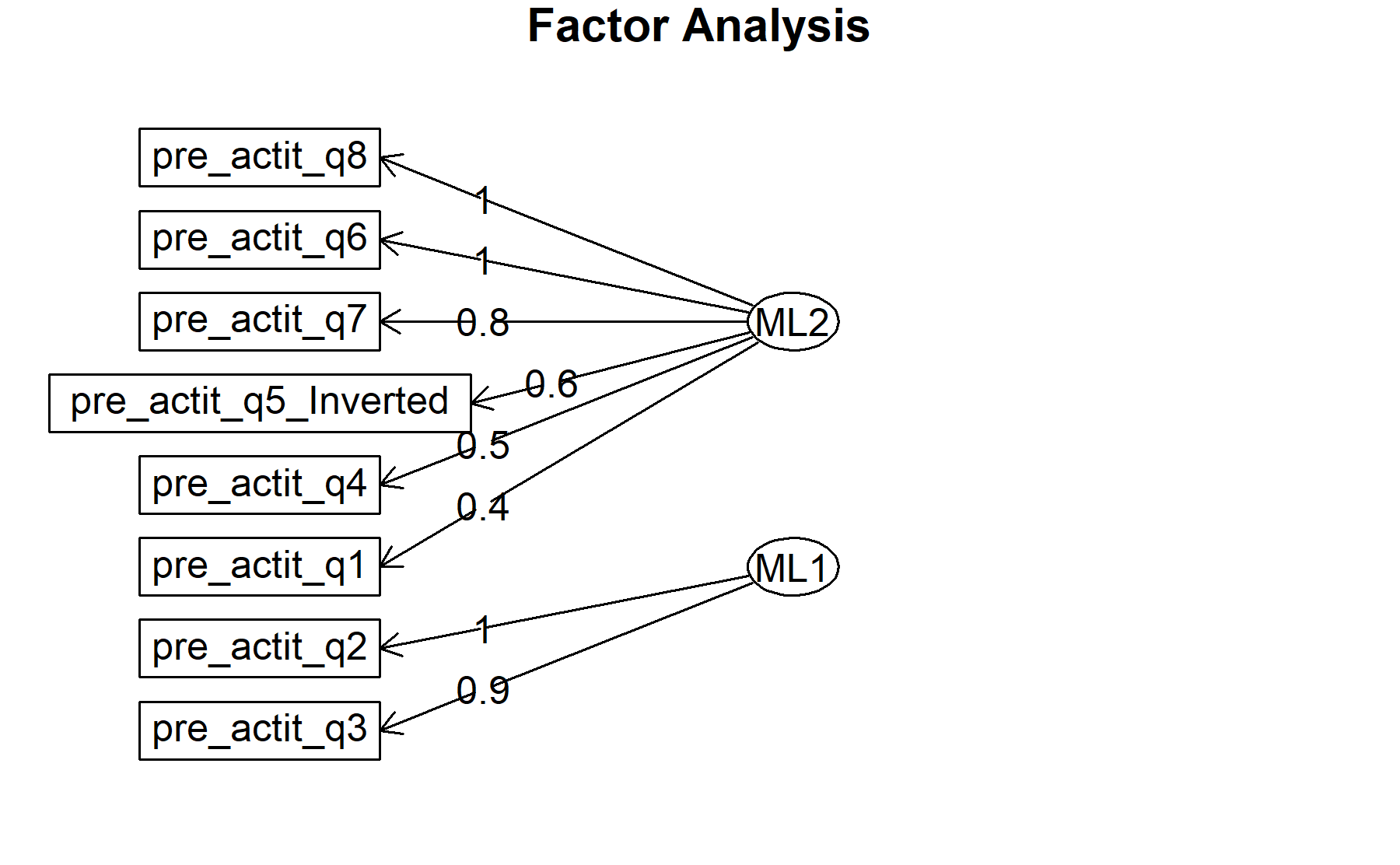
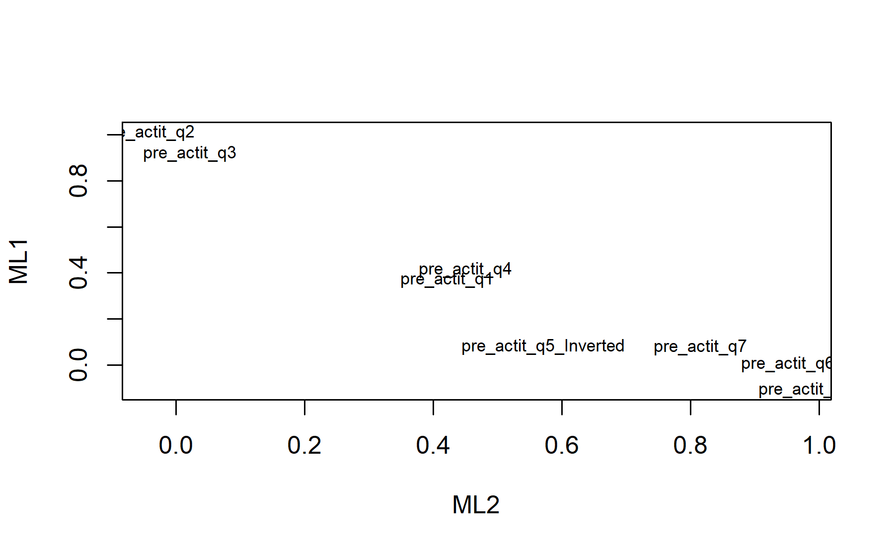
## Standardized loadings (pattern matrix) based upon correlation matrix
## ML2 ML1 h2 u2 com
## pre_actit_q1 0.42 0.42 0.576 2
## pre_actit_q2 1.01 1.00 0.005 1
## pre_actit_q3 0.92 0.86 0.138 1
## pre_actit_q4 0.45 0.42 0.50 0.497 2
## pre_actit_q6 0.95 0.91 0.091 1
## pre_actit_q7 0.82 0.72 0.285 1
## pre_actit_q8 0.98 0.90 0.103 1
## pre_actit_q5_Inverted 0.57 0.36 0.636 1
##
## ML2 ML1
## SS loadings 3.35 2.32
## Proportion Var 0.42 0.29
## Cumulative Var 0.42 0.71
## Proportion Explained 0.59 0.41
## Cumulative Proportion 0.59 1.00
##
## With factor correlations of
## ML2 ML1
## ML2 1.00 0.34
## ML1 0.34 1.00
##
## Mean item complexity = 1.3
## Test of the hypothesis that 2 factors are sufficient.
##
## df null model = 28 with the objective function = 29.11 with Chi Square = 1237
## df of the model are 13 and the objective function was 22.61
##
## The root mean square of the residuals (RMSR) is 0.11
## The df corrected root mean square of the residuals is 0.16
##
## The harmonic n.obs is 47 with the empirical chi square 30.08 with prob < 0.0046
## The total n.obs was 47 with Likelihood Chi Square = 930.9 with prob < 1.2e-190
##
## Tucker Lewis Index of factoring reliability = -0.689
## RMSEA index = 1.225 and the 90 % confidence intervals are 1.172 1.307
## BIC = 880.8
## Fit based upon off diagonal values = 0.96
## Measures of factor score adequacy
## ML2 ML1
## Correlation of (regression) scores with factors 0.98 1.00
## Multiple R square of scores with factors 0.96 1.00
## Minimum correlation of possible factor scores 0.92 0.99Exploring these results, there are two factors composed by:
ML1: Q1, Q4, Q6, Q7, Q8, Q5 inv.
ML2: Q2, Q3, Q4.
Finally, plots show the relationship between the items and the factors.
10.2.2 Excluding item 4 (preserving item 5 inverted)..
First, a factor analysis with all the 7 items is performed.
As first approach the Barlett’s sphericity test is performed.
Thus, the p-value = 0 and the H0 is rejected confirming the utility of applying a factor analysis to this dataset.
Considering the fact that the Bartlett’s test usually rejects the H0 since the scenario of the null hypothesis is too extreme, the KMO analysis is studied to determine how well the data fit the factor analysis and how useful each item is.
## Kaiser-Meyer-Olkin factor adequacy
## Call: KMO(r = pre_test_Q_Actitd_facAn_2_corr)
## Overall MSA =  0.56
## MSA for each item =
##     q1     q2     q3     q6     q7     q8 q5_Inv
##   0.48   0.52   0.54   0.60   0.57   0.61   0.81
According to these results, there is one items under the threshold of 0.5 (Q1=0.48). Three items are below 0.6.
To explore the number of factors PCA and evaluate the variability explained for each component is considered. Thus, the table with the PCA results is shown below:
| PC1 | PC2 | PC3 | PC4 | PC5 | PC6 | PC7 | |
|---|---|---|---|---|---|---|---|
| Standard deviation | 1.7045 | 1.2634 | 1.1311 | 0.8474 | 0.5389 | 0.3363 | 0.3117 |
| Proportion of Variance | 0.4151 | 0.2280 | 0.1828 | 0.1026 | 0.0415 | 0.0162 | 0.0139 |
| Cumulative Proportion | 0.4151 | 0.6431 | 0.8259 | 0.9285 | 0.9700 | 0.9861 | 1.0000 |
Then, the scree plot for this PCA analysis is displayed.
 According to these results, with two 64% of the variability is explained and the elbow on the second component.
Then, another approach is implemented. With this strategy several analysis are combined and depict in the same figure. The tools implemented are: the Kaiser rule (which drops the components with eigenvalues < 1), the parallel analysis, and the usual scree test (plotuScree), the acceleration factor (which indicates where the elbow of the scree plot appears).
 Therefore, two factors will be considered.
Running the factor analysis with all the items (n=7), first the communalities are explored:
##          pre_actit_q1          pre_actit_q2          pre_actit_q3
##                0.4034                0.9950                0.9110
##          pre_actit_q6          pre_actit_q7          pre_actit_q8
##                0.9114                0.7057                0.9057
## pre_actit_q5_Inverted
##                0.3667
Therefore, considering the values of the communalities, only the Q5 inverted is under 0.4.
Then, the whole output is displayed.
## Factor Analysis using method =  ml
## Call: fa(r = pre_test_Q_Actitd_facAn_2, nfactors = 2, rotate = "oblimin",
##     fm = "ml", cor = "poly")
## Standardized loadings (pattern matrix) based upon correlation matrix
##                         ML2   ML1   h2    u2 com
## pre_actit_q1           0.41       0.40 0.597 2.0
## pre_actit_q2                 1.01 1.00 0.005 1.0
## pre_actit_q3                 0.94 0.91 0.089 1.0
## pre_actit_q6           0.95       0.91 0.089 1.0
## pre_actit_q7           0.80       0.71 0.294 1.0
## pre_actit_q8           0.98       0.91 0.094 1.0
## pre_actit_q5_Inverted  0.57       0.37 0.633 1.1
##
##                        ML2  ML1
## SS loadings           3.06 2.14
## Proportion Var        0.44 0.31
## Cumulative Var        0.44 0.74
## Proportion Explained  0.59 0.41
## Cumulative Proportion 0.59 1.00
##
##  With factor correlations of
##      ML2  ML1
## ML2 1.00 0.32
## ML1 0.32 1.00
##
## Mean item complexity =  1.2
## Test of the hypothesis that 2 factors are sufficient.
##
## df null model =  21  with the objective function =  8.41 with Chi Square =  360.3
## df of  the model are 8  and the objective function was  2.17
##
## The root mean square of the residuals (RMSR) is  0.09
## The df corrected root mean square of the residuals is  0.14
##
## The harmonic n.obs is  47 with the empirical chi square  14.58  with prob <  0.068
## The total n.obs was  47  with Likelihood Chi Square =  89.88  with prob <  0.00000000000000049
##
## Tucker Lewis Index of factoring reliability =  0.345
## RMSEA index =  0.466  and the 90 % confidence intervals are  0.387 0.562
## BIC =  59.08
## Fit based upon off diagonal values = 0.98
## Measures of factor score adequacy
##                                                    ML2  ML1
## Correlation of (regression) scores with factors   0.98 1.00
## Multiple R square of scores with factors          0.96 1.00
## Minimum correlation of possible factor scores     0.92 0.99
Exploring these results, there are two factors composed by:
* Q1, Q6, Q7, Q8, and Q5 inv.
* Q2, and Q3.
Finally, plots show the relationship between the items and the factors.
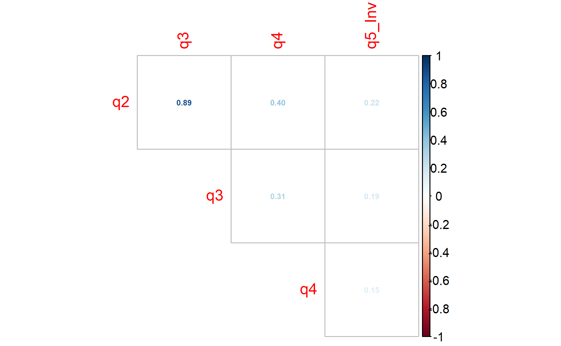
10.2.3 Including Q2, Q3, Q4 and Q5 inverted.
First, a factor analysis with all the 4 items is performed.
As first approach the Barlett’s sphericity test is performed.
Thus, the p-value = 0 and the H0 is rejected confirming the utility of applying a factor analysis to this dataset.
Considering the fact that the Bartlett’s test usually rejects the H0 since the scenario of the null hypothesis is too extreme, the KMO analysis is studied to determine how well the data fit the factor analysis and how useful each item is.
## Kaiser-Meyer-Olkin factor adequacy
## Call: KMO(r = pre_test_Q_Actitd_facAn_3_corr)
## Overall MSA =  0.57
## MSA for each item =
##     q2     q3     q4 q5_Inv
##   0.54   0.54   0.76   0.88
According to these results, all the items are above 0.5. Two items are below 0.6.
To explore the number of factors PCA and evaluate the variability explained for each component is considered. Thus, the table with the PCA results is shown below:
| PC1 | PC2 | PC3 | PC4 | |
|---|---|---|---|---|
| Standard deviation | 1.4835 | 0.9563 | 0.8816 | 0.3280 |
| Proportion of Variance | 0.5502 | 0.2286 | 0.1943 | 0.0269 |
| Cumulative Proportion | 0.5502 | 0.7788 | 0.9731 | 1.0000 |
Then, the scree plot for this PCA analysis is displayed.
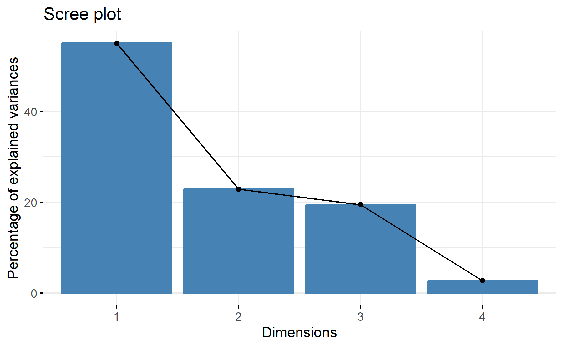 According to these results, one factor seems to be sufficient.
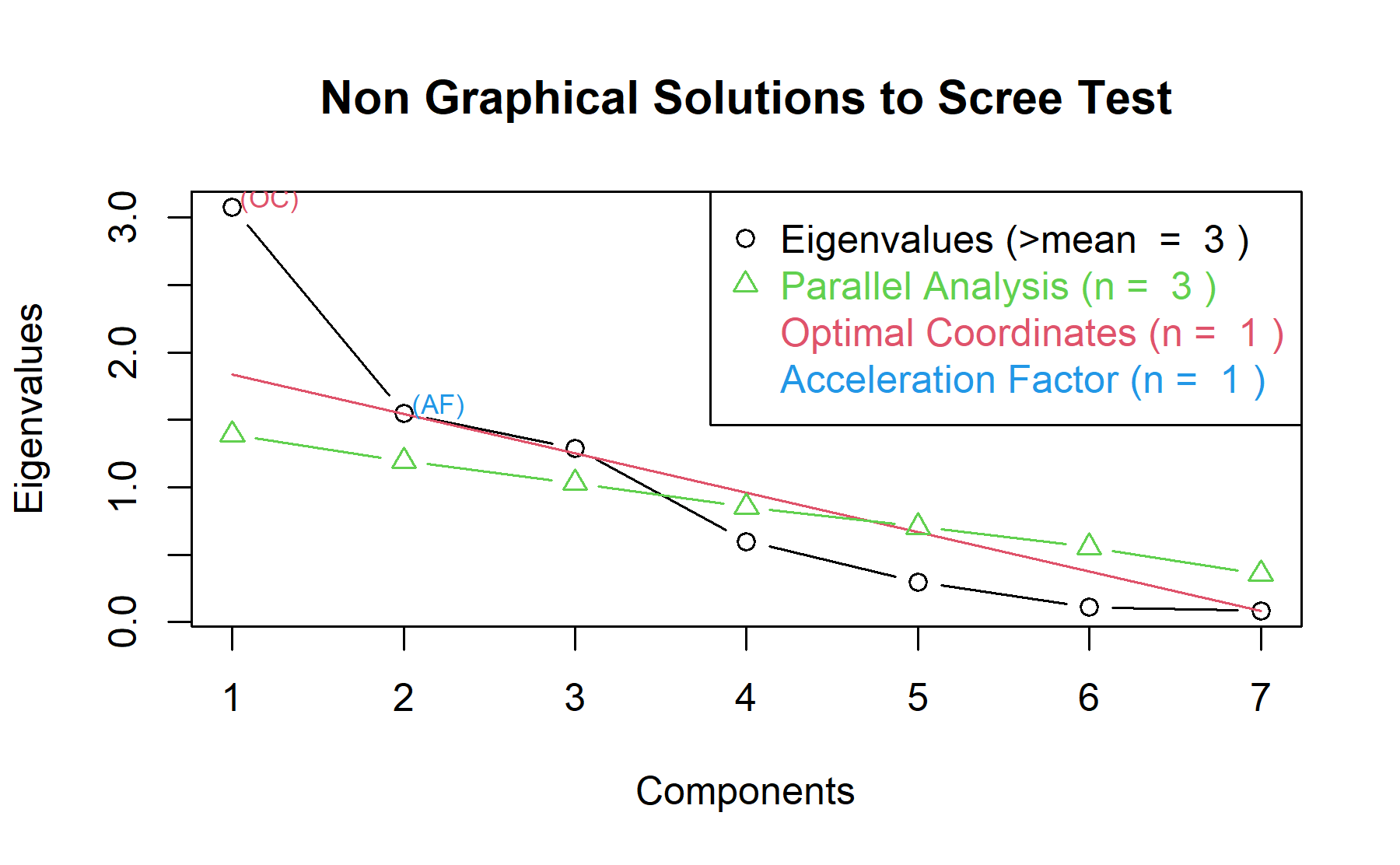
Then, another approach is implemented. With this strategy several analysis are combined and depict in the same figure. The tools implemented are: the Kaiser rule (which drops the components with eigenvalues < 1), the parallel analysis, and the usual scree test (plotuScree), the acceleration factor (which indicates where the elbow of the scree plot appears).
 Therefore, 1 factor will be considered.
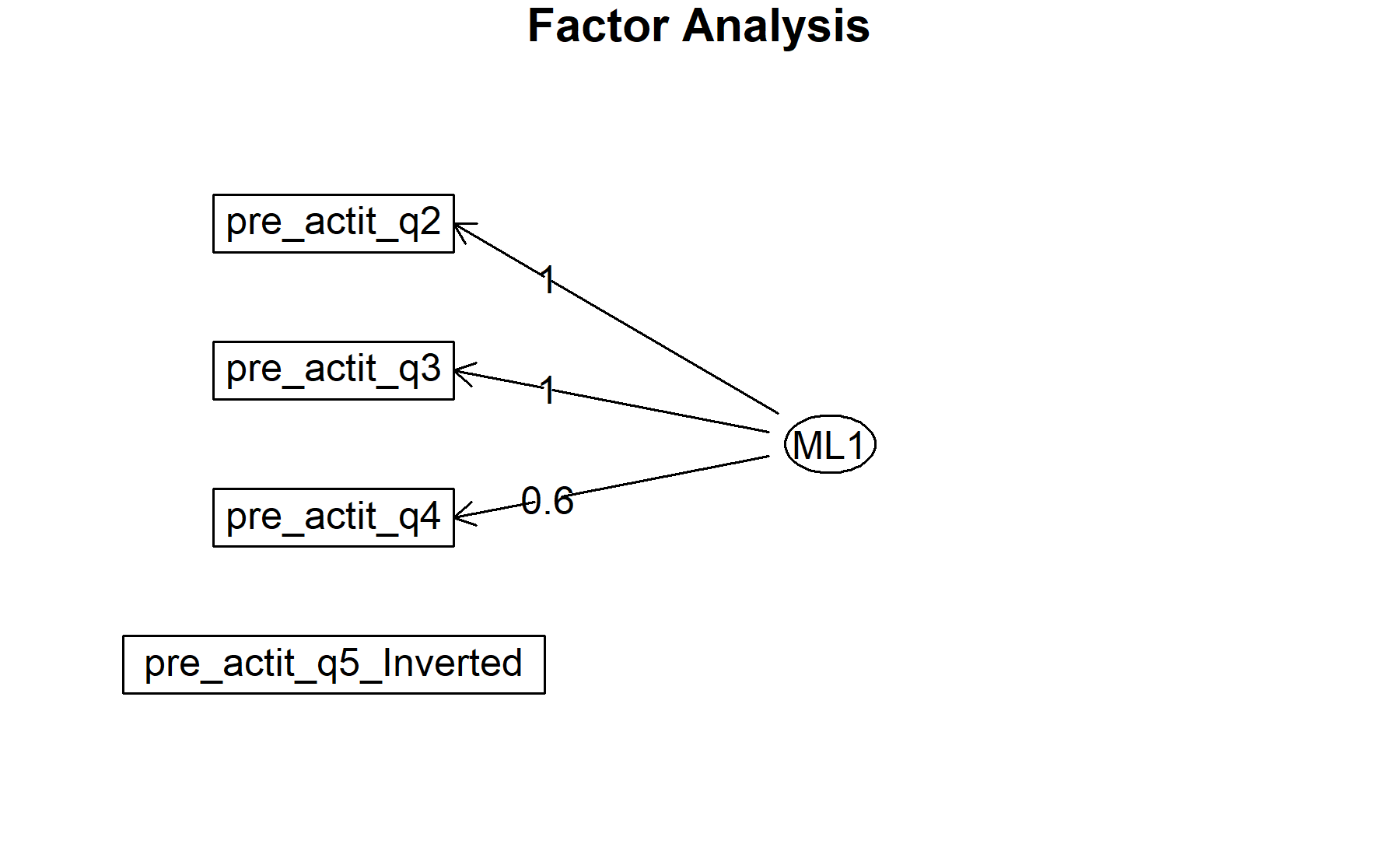
Running the factor analysis with all the items (n=4), first the communalities are explored:
##          pre_actit_q2          pre_actit_q3          pre_actit_q4
##               0.99500               0.90638               0.32037
## pre_actit_q5_Inverted
##               0.06679
Therefore, considering the values of the communalities, only the Q5 inverted is under 0.4.
Then, the whole output is displayed.
## Factor Analysis using method =  ml
## Call: fa(r = pre_test_Q_Actitd_facAn_3, nfactors = 1, rotate = "oblimin",
##     fm = "ml", cor = "poly")
## Standardized loadings (pattern matrix) based upon correlation matrix
##                        ML1    h2     u2 com
## pre_actit_q2          1.00 0.995 0.0049   1
## pre_actit_q3          0.95 0.906 0.0936   1
## pre_actit_q4          0.57 0.320 0.6796   1
## pre_actit_q5_Inverted      0.067 0.9332   1
##
##                 ML1
## SS loadings    2.29
## Proportion Var 0.57
##
## Mean item complexity =  1
## Test of the hypothesis that 1 factor is sufficient.
##
## df null model =  6  with the objective function =  3.06 with Chi Square =  134.2
## df of  the model are 2  and the objective function was  0.28
##
## The root mean square of the residuals (RMSR) is  0.07
## The df corrected root mean square of the residuals is  0.12
##
## The harmonic n.obs is  47 with the empirical chi square  2.7  with prob <  0.26
## The total n.obs was  47  with Likelihood Chi Square =  11.95  with prob <  0.0025
##
## Tucker Lewis Index of factoring reliability =  0.763
## RMSEA index =  0.325  and the 90 % confidence intervals are  0.167 0.519
## BIC =  4.25
## Fit based upon off diagonal values = 0.98
## Measures of factor score adequacy
##                                                    ML1
## Correlation of (regression) scores with factors   1.00
## Multiple R square of scores with factors          1.00
## Minimum correlation of possible factor scores     0.99
Exploring these results, there are two factors composed by:
ML1: Q2, Q3, Q4.
Out: Q5 inv.
Finally, plots show the relationship between the items and the factors.
10.2.4 Excluding item 5 (preserving item 4).
First, a factor analysis with all the 7 items is performed.
As first approach the Barlett’s sphericity test is performed.
Thus, the p-value = 0 and the H0 is rejected confirming the utility of applying a factor analysis to this dataset.
Considering the fact that the Bartlett’s test usually rejects the H0 since the scenario of the null hypothesis is too extreme, the KMO analysis is studied to determine how well the data fit the factor analysis and how useful each item is.
## Kaiser-Meyer-Olkin factor adequacy
## Call: KMO(r = pre_test_Q_Actitd_facAn_4_corr)
## Overall MSA =  0.55
## MSA for each item =
##   q1   q2   q3   q4   q6   q7   q8
## 0.47 0.51 0.53 0.66 0.57 0.57 0.58
According to these results, there is one items under the threshold of 0.5 (Q1=0.47). Five items are below 0.6.
To explore the number of factors PCA and evaluate the variability explained for each component is considered. Thus, the table with the PCA results is shown below:
| PC1 | PC2 | PC3 | PC4 | PC5 | PC6 | PC7 | |
|---|---|---|---|---|---|---|---|
| Standard deviation | 1.7538 | 1.2435 | 1.1348 | 0.7741 | 0.5451 | 0.3306 | 0.2907 |
| Proportion of Variance | 0.4394 | 0.2209 | 0.1840 | 0.0856 | 0.0424 | 0.0156 | 0.0121 |
| Cumulative Proportion | 0.4394 | 0.6603 | 0.8442 | 0.9299 | 0.9723 | 0.9879 | 1.0000 |
Then, the scree plot for this PCA analysis is displayed.
 According to these results, with two 66% of the variability is explained, while with three 84%; besides, there is an elbow on the second and on the third component.
Then, another approach is implemented. With this strategy several analysis are combined and depict in the same figure. The tools implemented are: the Kaiser rule (which drops the components with eigenvalues < 1), the parallel analysis, and the usual scree test (plotuScree), the acceleration factor (which indicates where the elbow of the scree plot appears).
 Therefore, two factors will be considered.
Running the factor analysis with all the items (n=7), first the communalities are explored:
## Warning in cor.smooth(mat): Matrix was not positive definite, smoothing was
## done
## In factor.stats, I could not find the RMSEA upper bound . Sorry about that## pre_actit_q1 pre_actit_q2 pre_actit_q3 pre_actit_q4 pre_actit_q6 pre_actit_q7
## 0.4172 0.9950 0.8776 0.5091 0.9044 0.6907
## pre_actit_q8
## 0.9154Therefore, considering the values of the communalities, all of them are above 0.4.
Then, the whole output is displayed.
## Factor Analysis using method =  ml
## Call: fa(r = pre_test_Q_Actitd_facAn_4, nfactors = 2, rotate = "oblimin",
##     fm = "ml", cor = "poly")
## Standardized loadings (pattern matrix) based upon correlation matrix
##                ML2   ML1   h2    u2 com
## pre_actit_q1  0.41       0.42 0.583   2
## pre_actit_q2        1.01 1.00 0.005   1
## pre_actit_q3        0.93 0.88 0.122   1
## pre_actit_q4  0.45  0.43 0.51 0.490   2
## pre_actit_q6  0.95       0.90 0.096   1
## pre_actit_q7  0.80       0.69 0.309   1
## pre_actit_q8  0.99       0.92 0.085   1
##
##                        ML2  ML1
## SS loadings           2.98 2.33
## Proportion Var        0.43 0.33
## Cumulative Var        0.43 0.76
## Proportion Explained  0.56 0.44
## Cumulative Proportion 0.56 1.00
##
##  With factor correlations of
##      ML2  ML1
## ML2 1.00 0.33
## ML1 0.33 1.00
##
## Mean item complexity =  1.3
## Test of the hypothesis that 2 factors are sufficient.
##
## df null model =  21  with the objective function =  28.24 with Chi Square =  1209
## df of  the model are 8  and the objective function was  22.04
##
## The root mean square of the residuals (RMSR) is  0.11
## The df corrected root mean square of the residuals is  0.18
##
## The harmonic n.obs is  47 with the empirical chi square  25.1  with prob <  0.0015
## The total n.obs was  47  with Likelihood Chi Square =  914.7  with prob <  3.7e-192
##
## Tucker Lewis Index of factoring reliability =  -1.068
## RMSEA index =  1.553  and the 90 % confidence intervals are  1.485 NA
## BIC =  883.9
## Fit based upon off diagonal values = 0.96
## Measures of factor score adequacy
##                                                    ML2  ML1
## Correlation of (regression) scores with factors   0.98 1.00
## Multiple R square of scores with factors          0.96 1.00
## Minimum correlation of possible factor scores     0.92 0.99
Exploring these results, there are two factors composed by:
ML2: Q1, Q4, Q6, Q7, and Q8.
ML2: Q2, Q3, and Q4.
Finally, plots show the relationship between the items and the factors.
10.2.5 Conclusions
Item Q1 did not show association with Q2 and Q3, indeed, this was grouped with motivations (Q6-8). Q4 was found linked with both factors.
Item Q5 inverted, when was included with motivation questions it grouped with them.
Therefore, Q1 could be excluded at least from factor analysis. Q4 and Q5 could be tested with the remaining items to performed a wider factor analysis.
10.3 Both domains, the expectations and concerns domain plus the attitudes domain
10.3.1 Expectations plus Q2 and Q3 from attitudes.
Including all the items selected for expectations (Q2, Q5, Q6, Q7.i, Q7.iv, Q7.v, Q8, Q9, 10, and Q11), plus two items from the attitude domain (Q2 and Q3).
The Barlett’s sphericity test is performed.
Thus, the p-value = 0 and the H0 is rejected confirming the utility of applying a factor analysis to this dataset.
Considering the fact that the Bartlett’s test usually rejects the H0 since the scenario of the null hypothesis is too extreme, the KMO analysis is studied to determine how well the data fit the factor analysis and how useful each item is.
## Kaiser-Meyer-Olkin factor adequacy
## Call: KMO(r = pre_test_Q_Exp_Attit_facAn_1_corr)
## Overall MSA =  0.56
## MSA for each item =
##       q2       q5       q6     q7_i    q7_iv     q7_v       q8       q9
##     0.53     0.74     0.52     0.64     0.63     0.67     0.49     0.49
##      q10      q11 actit_q2 actit_q3
##     0.62     0.51     0.54     0.54
According to these results, there are two items under the threshold of 0.5 (Q8 and Q9 with 0.49). Five items are below 0.6.
To explore the number of factors PCA is applied. Thus, the table with the PCA results is shown below:
| PC1 | PC2 | PC3 | PC4 | PC5 | PC6 | PC7 | PC8 | PC9 | PC10 | PC11 | PC12 | |
|---|---|---|---|---|---|---|---|---|---|---|---|---|
| Standard deviation | 1.8031 | 1.6163 | 1.3617 | 1.0426 | 0.9009 | 0.8182 | 0.7502 | 0.7200 | 0.5259 | 0.4189 | 0.3104 | 0.2907 |
| Proportion of Variance | 0.2709 | 0.2177 | 0.1545 | 0.0906 | 0.0676 | 0.0558 | 0.0469 | 0.0432 | 0.0231 | 0.0146 | 0.0080 | 0.0070 |
| Cumulative Proportion | 0.2709 | 0.4886 | 0.6432 | 0.7337 | 0.8014 | 0.8572 | 0.9041 | 0.9473 | 0.9703 | 0.9849 | 0.9930 | 1.0000 |
Then, the scree plot for this PCA analysis is displayed.
 According to these results, 3-4 factors could be the best number. The cumulative proportion showed that with 3 components 64% of the variance could be explained and with four it is 73%. The elbow seems to be on the four component.
Then, another approach is implemented. With this strategy several analysis are combined and depict in the same figure. The tools implemented are: the Kaiser rule (which drops the components with eigenvalues < 1), the parallel analysis, and the usual scree test (plotuScree), the acceleration factor (which indicates where the elbow of the scree plot appears).
 Therefore, considering three factors seem to be an adequate approach.
Running the factor analysis with 12 items, first the communalities are explored:
## Warning in cor.smooth(mat): Matrix was not positive definite, smoothing was
## done
## pre_exp_preoc_q2 pre_exp_preoc_q5 pre_exp_preoc_q6 pre_exp_preoc_q7_i
## 0.4866 0.3529 0.6369 0.3329
## pre_exp_preoc_q7_iv pre_exp_preoc_q7_v pre_exp_preoc_q8 pre_exp_preoc_q9
## 0.9950 0.8775 0.6098 0.9950
## pre_exp_preoc_q10 pre_exp_preoc_q11 pre_actit_q2 pre_actit_q3
## 0.1939 0.4646 0.9950 0.9054Considering the values of the communalities, Q10 is under 0.3.
Then, the whole output is displayed.
## Factor Analysis using method =  ml
## Call: fa(r = pre_test_Q_Exp_Attit_facAn_1, nfactors = 3, rotate = "oblimin",
##     fm = "ml", cor = "poly")
## Standardized loadings (pattern matrix) based upon correlation matrix
##                       ML2   ML3   ML1   h2     u2 com
## pre_exp_preoc_q2          -0.70       0.49 0.5134 1.1
## pre_exp_preoc_q5     0.57             0.35 0.6472 1.2
## pre_exp_preoc_q6     0.72             0.64 0.3636 1.2
## pre_exp_preoc_q7_i   0.45             0.33 0.6679 1.7
## pre_exp_preoc_q7_iv  1.01             1.00 0.0049 1.0
## pre_exp_preoc_q7_v   0.89             0.88 0.1225 1.1
## pre_exp_preoc_q8           0.75       0.61 0.3902 1.0
## pre_exp_preoc_q9           1.00       1.00 0.0050 1.0
## pre_exp_preoc_q10          0.44       0.19 0.8061 1.2
## pre_exp_preoc_q11          0.49       0.46 0.5352 2.4
## pre_actit_q2                     1.00 1.00 0.0050 1.0
## pre_actit_q3                     0.94 0.91 0.0946 1.0
##
##                        ML2  ML3  ML1
## SS loadings           2.98 2.63 2.23
## Proportion Var        0.25 0.22 0.19
## Cumulative Var        0.25 0.47 0.65
## Proportion Explained  0.38 0.33 0.28
## Cumulative Proportion 0.38 0.72 1.00
##
##  With factor correlations of
##       ML2   ML3   ML1
## ML2  1.00 -0.15  0.14
## ML3 -0.15  1.00 -0.22
## ML1  0.14 -0.22  1.00
##
## Mean item complexity =  1.3
## Test of the hypothesis that 3 factors are sufficient.
##
## df null model =  66  with the objective function =  33.46 with Chi Square =  1310
## df of  the model are 33  and the objective function was  24.76
##
## The root mean square of the residuals (RMSR) is  0.11
## The df corrected root mean square of the residuals is  0.15
##
## The harmonic n.obs is  45 with the empirical chi square  69.14  with prob <  0.00023
## The total n.obs was  45  with Likelihood Chi Square =  920.1  with prob <  5.8e-172
##
## Tucker Lewis Index of factoring reliability =  -0.507
## RMSEA index =  0.773  and the 90 % confidence intervals are  0.739 0.826
## BIC =  794.5
## Fit based upon off diagonal values = 0.91
## Measures of factor score adequacy
##                                                    ML2  ML3  ML1
## Correlation of (regression) scores with factors   1.00 1.00 1.00
## Multiple R square of scores with factors          1.00 1.00 1.00
## Minimum correlation of possible factor scores     0.99 0.99 0.99
There are 3 factors:
* Q2, Q8, Q9, Q10, Q11.
* Q5, Q6, Q7_i, Q7_iv, Q7_v.
* attQ2, attQ3
Finally, plots show the relationship between the items and the factors.
10.3.2 Expectations plus Q2, Q3, and Q4 from attitudes.
Including all the items selected for expectations (Q2, Q5, Q6, Q7.i, Q7.iv, Q7.v, Q8, Q9, 10, and Q11), plus three items from the attitude domain (Q2, Q3, and Q4).
The Barlett’s sphericity test is performed.
Thus, the p-value = 0 and the H0 is rejected confirming the utility of applying a factor analysis to this dataset.
Considering the fact that the Bartlett’s test usually rejects the H0 since the scenario of the null hypothesis is too extreme, the KMO analysis is studied to determine how well the data fit the factor analysis and how useful each item is.
## Kaiser-Meyer-Olkin factor adequacy
## Call: KMO(r = pre_test_Q_Exp_Attit_facAn_2_corr)
## Overall MSA =  0.56
## MSA for each item =
##       q2       q5       q6     q7_i    q7_iv     q7_v       q8       q9
##     0.59     0.74     0.59     0.55     0.67     0.69     0.50     0.49
##      q10      q11 actit_q2 actit_q3 actit_q4
##     0.60     0.45     0.48     0.54     0.58
According to these results, there are items under the threshold of 0.5 (Q9, Q11, attQ2). Six item are below 0.6.
To explore the number of factors PCA is applied. Thus, the table with the PCA results is shown below:
| PC1 | PC2 | PC3 | PC4 | PC5 | PC6 | PC7 | PC8 | PC9 | PC10 | PC11 | PC12 | PC13 | |
|---|---|---|---|---|---|---|---|---|---|---|---|---|---|
| Standard deviation | 1.8753 | 1.6472 | 1.3617 | 1.1061 | 0.9016 | 0.8865 | 0.7935 | 0.7209 | 0.5793 | 0.5239 | 0.4147 | 0.2949 | 0.2739 |
| Proportion of Variance | 0.2705 | 0.2087 | 0.1426 | 0.0941 | 0.0625 | 0.0605 | 0.0484 | 0.0400 | 0.0258 | 0.0211 | 0.0132 | 0.0067 | 0.0058 |
| Cumulative Proportion | 0.2705 | 0.4792 | 0.6219 | 0.7160 | 0.7785 | 0.8390 | 0.8874 | 0.9274 | 0.9532 | 0.9743 | 0.9875 | 0.9942 | 1.0000 |
Then, the scree plot for this PCA analysis is displayed.
 According to these results, 3-4 factors could be the best number. The cumulative proportion showed that with 3 components 62% and 72% with four. The greatest elbow is on the four component.
Then, another approach is implemented. With this strategy several analysis are combined and depict in the same figure. The tools implemented are: the Kaiser rule (which drops the components with eigenvalues < 1), the parallel analysis, and the usual scree test (plotuScree), the acceleration factor (which indicates where the elbow of the scree plot appears).
 Therefore, considering three factors seem to be an adequate approach.
Running the factor analysis with 13 items, first the communalities are explored:
## Warning in cor.smooth(mat): Matrix was not positive definite, smoothing was
## done
## In factor.stats, I could not find the RMSEA upper bound . Sorry about that## pre_exp_preoc_q2 pre_exp_preoc_q5 pre_exp_preoc_q6 pre_exp_preoc_q7_i
## 0.5324 0.3713 0.6314 0.3676
## pre_exp_preoc_q7_iv pre_exp_preoc_q7_v pre_exp_preoc_q8 pre_exp_preoc_q9
## 0.9950 0.8785 0.5854 0.9080
## pre_exp_preoc_q10 pre_exp_preoc_q11 pre_actit_q2 pre_actit_q3
## 0.2004 0.4835 0.9950 0.8624
## pre_actit_q4
## 0.4851Considering the values of the communalities, Q10 is under 0.3.
Then, the whole output is displayed.
## Factor Analysis using method =  ml
## Call: fa(r = pre_test_Q_Exp_Attit_facAn_2, nfactors = 3, rotate = "oblimin",
##     fm = "ml", cor = "poly")
## Standardized loadings (pattern matrix) based upon correlation matrix
##                       ML1   ML3   ML2   h2    u2 com
## pre_exp_preoc_q2          -0.73       0.53 0.467 1.1
## pre_exp_preoc_q5     0.57             0.37 0.633 1.3
## pre_exp_preoc_q6     0.72             0.63 0.369 1.2
## pre_exp_preoc_q7_i   0.44             0.37 0.632 1.9
## pre_exp_preoc_q7_iv  1.01             1.00 0.005 1.1
## pre_exp_preoc_q7_v   0.89             0.88 0.121 1.1
## pre_exp_preoc_q8           0.74       0.59 0.414 1.0
## pre_exp_preoc_q9           0.95       0.91 0.092 1.0
## pre_exp_preoc_q10          0.45       0.21 0.793 1.2
## pre_exp_preoc_q11          0.53       0.48 0.516 2.3
## pre_actit_q2                     1.00 1.00 0.005 1.0
## pre_actit_q3                     0.91 0.86 0.138 1.0
## pre_actit_q4         0.55             0.49 0.513 1.8
##
##                        ML1  ML3  ML2
## SS loadings           3.32 2.67 2.31
## Proportion Var        0.26 0.21 0.18
## Cumulative Var        0.26 0.46 0.64
## Proportion Explained  0.40 0.32 0.28
## Cumulative Proportion 0.40 0.72 1.00
##
##  With factor correlations of
##       ML1   ML3   ML2
## ML1  1.00 -0.13  0.16
## ML3 -0.13  1.00 -0.20
## ML2  0.16 -0.20  1.00
##
## Mean item complexity =  1.3
## Test of the hypothesis that 3 factors are sufficient.
##
## df null model =  78  with the objective function =  54.7 with Chi Square =  2124
## df of  the model are 42  and the objective function was  45.82
##
## The root mean square of the residuals (RMSR) is  0.11
## The df corrected root mean square of the residuals is  0.15
##
## The harmonic n.obs is  45 with the empirical chi square  84.49  with prob <  0.00011
## The total n.obs was  45  with Likelihood Chi Square =  1688  with prob <  0
##
## Tucker Lewis Index of factoring reliability =  -0.578
## RMSEA index =  0.933  and the 90 % confidence intervals are  0.905 NA
## BIC =  1528
## Fit based upon off diagonal values = 0.91
## Measures of factor score adequacy
##                                                    ML1  ML3  ML2
## Correlation of (regression) scores with factors   1.00 0.97 1.00
## Multiple R square of scores with factors          1.00 0.93 1.00
## Minimum correlation of possible factor scores     0.99 0.86 0.99
There are 3 factors:
* attQ2, attQ3.
* Q5, Q6, Q7_i, Q7_iv, Q7_v, attQ4.
* Q8, Q9, Q10, Q11, Q2.
Finally, plots show the relationship between the items and the factors.

10.3.3 Expectations plus Q2, Q3, Q4, and Q5 from attitudes.
Including all the items selected for expectations (Q2, Q5, Q6, Q7.i, Q7.iv, Q7.v, Q8, Q9, 10, and Q11), plus four items from the attitude domain (Q2, Q3, Q4, and Q5 inverted).
The Barlett’s sphericity test is performed.
Thus, the p-value = 0 and the H0 is rejected confirming the utility of applying a factor analysis to this dataset.
Considering the fact that the Bartlett’s test usually rejects the H0 since the scenario of the null hypothesis is too extreme, the KMO analysis is studied to determine how well the data fit the factor analysis and how useful each item is.
## Kaiser-Meyer-Olkin factor adequacy
## Call: KMO(r = pre_test_Q_Exp_Attit_facAn_3_corr)
## Overall MSA =  0.56
## MSA for each item =
##           q2           q5           q6         q7_i        q7_iv         q7_v
##         0.65         0.61         0.62         0.58         0.69         0.68
##           q8           q9          q10          q11     actit_q2     actit_q3
##         0.49         0.52         0.65         0.47         0.44         0.51
##     actit_q4 actit_q5_Inv
##         0.53         0.55
According to these results, there are items under the threshold of 0.5 (Q8, Q11, attQ2). Five item are below 0.6.
To explore the number of factors PCA is applied. Thus, the table with the PCA results is shown below:
| PC1 | PC2 | PC3 | PC4 | PC5 | PC6 | PC7 | PC8 | PC9 | PC10 | PC11 | PC12 | PC13 | PC14 | |
|---|---|---|---|---|---|---|---|---|---|---|---|---|---|---|
| Standard deviation | 1.9470 | 1.6753 | 1.3682 | 1.1143 | 0.9033 | 0.8928 | 0.8675 | 0.7833 | 0.6888 | 0.5786 | 0.4366 | 0.4038 | 0.2923 | 0.2478 |
| Proportion of Variance | 0.2708 | 0.2005 | 0.1337 | 0.0887 | 0.0583 | 0.0569 | 0.0538 | 0.0438 | 0.0339 | 0.0239 | 0.0136 | 0.0117 | 0.0061 | 0.0044 |
| Cumulative Proportion | 0.2708 | 0.4712 | 0.6050 | 0.6936 | 0.7519 | 0.8089 | 0.8626 | 0.9064 | 0.9403 | 0.9642 | 0.9779 | 0.9895 | 0.9956 | 1.0000 |
Then, the scree plot for this PCA analysis is displayed.
 According to these results, 3-4 factors could be the best number. There is not a clear elbow. The cumulative proportion showed that with 3 components 61% and 69% with four. The greatest elbow is on the four component.
Then, another approach is implemented. With this strategy several analysis are combined and depict in the same figure. The tools implemented are: the Kaiser rule (which drops the components with eigenvalues < 1), the parallel analysis, and the usual scree test (plotuScree), the acceleration factor (which indicates where the elbow of the scree plot appears).
 Therefore, considering three factors seem to be an adequate approach.
Running the factor analysis with 14 items, first the communalities are explored:
## Warning in cor.smooth(mat): Matrix was not positive definite, smoothing was
## done
## In factor.stats, I could not find the RMSEA upper bound . Sorry about that## pre_exp_preoc_q2 pre_exp_preoc_q5 pre_exp_preoc_q6
## 0.4916 0.3470 0.6377
## pre_exp_preoc_q7_i pre_exp_preoc_q7_iv pre_exp_preoc_q7_v
## 0.3332 0.9950 0.8703
## pre_exp_preoc_q8 pre_exp_preoc_q9 pre_exp_preoc_q10
## 0.5824 0.9950 0.1973
## pre_exp_preoc_q11 pre_actit_q2 pre_actit_q3
## 0.4409 0.9950 0.8543
## pre_actit_q4 pre_actit_q5_Inverted
## 0.4820 0.4660Considering the values of the communalities, Q10 is under 0.3.
Then, the whole output is displayed.
## Factor Analysis using method =  ml
## Call: fa(r = pre_test_Q_Exp_Attit_facAn_3, nfactors = 3, rotate = "oblimin",
##     fm = "ml", cor = "poly")
## Standardized loadings (pattern matrix) based upon correlation matrix
##                         ML2   ML3   ML1   h2    u2 com
## pre_exp_preoc_q2            -0.71       0.49 0.507 1.1
## pre_exp_preoc_q5       0.56             0.35 0.655 1.2
## pre_exp_preoc_q6       0.72             0.64 0.363 1.2
## pre_exp_preoc_q7_i     0.44             0.33 0.667 1.8
## pre_exp_preoc_q7_iv    1.01             1.00 0.005 1.1
## pre_exp_preoc_q7_v     0.89             0.87 0.129 1.1
## pre_exp_preoc_q8             0.74       0.58 0.417 1.0
## pre_exp_preoc_q9             1.00       1.00 0.005 1.0
## pre_exp_preoc_q10            0.44       0.20 0.805 1.2
## pre_exp_preoc_q11            0.49       0.44 0.559 2.4
## pre_actit_q2                       1.00 1.00 0.005 1.0
## pre_actit_q3                       0.91 0.85 0.145 1.0
## pre_actit_q4           0.55             0.48 0.517 1.8
## pre_actit_q5_Inverted       -0.60       0.47 0.533 1.2
##
##                        ML2  ML3  ML1
## SS loadings           3.36 3.01 2.32
## Proportion Var        0.24 0.22 0.17
## Cumulative Var        0.24 0.46 0.62
## Proportion Explained  0.39 0.35 0.27
## Cumulative Proportion 0.39 0.73 1.00
##
##  With factor correlations of
##       ML2   ML3   ML1
## ML2  1.00 -0.17  0.16
## ML3 -0.17  1.00 -0.21
## ML1  0.16 -0.21  1.00
##
## Mean item complexity =  1.3
## Test of the hypothesis that 3 factors are sufficient.
##
## df null model =  91  with the objective function =  74.06 with Chi Square =  2851
## df of  the model are 52  and the objective function was  64.65
##
## The root mean square of the residuals (RMSR) is  0.11
## The df corrected root mean square of the residuals is  0.15
##
## The harmonic n.obs is  45 with the empirical chi square  106.2  with prob <  0.000014
## The total n.obs was  45  with Likelihood Chi Square =  2360  with prob <  0
##
## Tucker Lewis Index of factoring reliability =  -0.546
## RMSEA index =  0.993  and the 90 % confidence intervals are  0.97 NA
## BIC =  2162
## Fit based upon off diagonal values = 0.9
## Measures of factor score adequacy
##                                                    ML2  ML3  ML1
## Correlation of (regression) scores with factors   1.00 1.00 1.00
## Multiple R square of scores with factors          1.00 1.00 1.00
## Minimum correlation of possible factor scores     0.99 0.99 0.99
There are 3 factors:
* attQ2, attQ3.
* Q5, Q6, Q7_i, Q7_iv, Q7_v, attQ4.
* Q8, Q9, Q10, Q11, -Q2, -attQ5.
Finally, plots show the relationship between the items and the factors.
10.3.4 Evaluating the presence of outliers
As an exploratory approach, the possibility of being a patient that answered all the items with “totally agree” is analyzed. Considering the small number of patients, and some behavior of the items along with the lack of complementary with the HOPE study with possibility is considered.
First, the existence of cases with this pattern is checked.
There is no patients with all the items (expectations plus attitudes), nor expectations items with a category 5 (totally agree) in their answers.
10.4 Final conclusion
According to the factor analysis the best approach is with:
Expectations and concerns: Q2, Q5, Q6, Q7_i, Q7_iv, Q7_v, Q8, Q9, Q10, Q11 (expectations: 6 items, concerns: 4)
Attitudes: Q2 and Q3.
Other items will be included: Q7_iii and Q3 from expectations, and Q9 as multiple choice element.
Additionally, there are two more items from attitudes: Q4 and Q5 that could be included. They showed different results and a conflicting behavior in several steps, in this cohort and in the VHIO. While Q4 seems to be more robust between analysis and metrics (even more when cohorts were compared), item Q5 was grouped in the same factor in both cohorts, with concerns items.
Thus, there are 10 (expectations) + 2 (attitudes) + 2 other potential (Q4 and Q5 attitudes) + 3 (not including in factor analysis) = 17 items.
Then, 2-3 items from sociodemographics, and 5 from knowledge.
Total: 24-25 items.